Anderson Insulators

An Anderson insulator has available single-particle states near the chemical potential, but those states are spatially localized and cannot sustain bulk diffusion at zero temperature. It can therefore be spectrally gapless and thermodynamically compressible while remaining electrically insulating. The obstruction is not absence of states; it is absence of extended transport paths.

At strictly zero temperature, a closed noninteracting Anderson insulator has vanishing dc conductivity in the thermodynamic limit. At nonzero temperature, localized carriers can move by exchanging energy with phonons or another environment. The resulting hopping conductivity is not a failure of localization. It is a dissipative transport channel between localized orbitals.

This page owns insulation without a band gap, the localized-orbital hopping picture, Miller–Abrahams networks, Mott variable-range hopping, the interaction-induced Coulomb gap, Efros–Shklovskii hopping, and experimental discrimination among those laws. Anderson Localization owns the microscopic localization mechanism and eigenstate diagnostics. Scaling Theory of Localization owns conductance beta functions and critical flow. Mobility Edges owns energy-resolved critical boundaries and their direct probes.

Regime and Convention Ledger

Quantity	Convention	Scope
Localization length	$\xi$ from exponential orbital tails	May depend on energy, disorder, and symmetry class
Single-particle density of states	$\rho(E)$ per volume and energy	Includes declared spin or valley degeneracy
Conductivity	$\sigma(T)$ in the low-field Ohmic regime	Prefactors can depend on temperature
Dielectric response	Relative permittivity $\kappa$	The Coulomb energy is $e^2/(4\pi\epsilon_0\kappa r)$
Localized-site energy	$\varepsilon_i$ measured relative to $\mu$ unless stated	Interactions renormalize addition and removal energies
Hopping environment	Equilibrated phonon bath unless stated	A closed static Hamiltonian cannot absorb an arbitrary energy mismatch
Disorder average	Typical or logarithmic transport statistic	Rare conducting paths can dominate arithmetic means

The canonical stretched-exponential form is

$$\sigma(T) = \sigma_0(T) \exp \left[ -\left( \frac{T_0}{T} \right)^p \right].$$

The exponent $p$ is only one part of a mechanism claim. Dimensionality, density of states, localization length, dielectric screening, prefactor, electric-field range, and temperature window must agree as well.

Insulation without a Band Gap

Density of states is not mobility

For extended diffusive carriers, the Einstein relation is

$$\sigma = e^2\rho(E_{\mathrm F})D.$$

An Anderson insulator can have

$$\rho(E_{\mathrm F})>0, \qquad D(E_{\mathrm F})=0,$$

and therefore

$$\sigma_{\mathrm{dc}}(0)=0.$$

The density of states counts available eigenvalues. The diffusion coefficient asks whether a wave packet spreads without bound. These are logically independent. A smooth tunneling spectrum does not prove metallic transport, and a divergent resistance does not prove a hard spectral gap.

For a sample of length $L$ with localized states at the Fermi energy, define a transport localization length $\xi_{\mathrm{tr}}$ through the typical coherent conductance:

$$\begin{aligned} g_{\mathrm{typ}}(L) &\equiv \exp\!\left[ \overline{\ln g(L)} \right], \\ \overline{\ln g(L)} &\sim -\frac{2L}{\xi_{\mathrm{tr}}}. \end{aligned}$$

Some authors absorb the factor of $2$ into $\xi_{\mathrm{tr}}$. Moreover, this estimator need not equal the orbital-tail length $\xi$ in a finite or multichannel geometry. The finite density of localized levels can still contribute to compressibility, heat capacity, optical absorption, local spectroscopy, and polarization. Those responses do not require dc charge to cross an infinite sample.

Distinguishing insulating mechanisms

Insulating regime	Low-energy states	Why dc transport is suppressed	Useful discriminator
Band insulator	Hard single-particle band gap	No bulk states at $\mu$	Band-resolved spectroscopy and activated carriers
Anderson insulator	Localized states may exist at $\mu$	Vanishing long-distance diffusion	Spatial localization, typical conductance, boundary sensitivity
Mott insulator	Interaction-driven charge gap or spectral-weight transfer	Charge addition is energetically costly	Many-body charge gap, Hubbard bands, local moments
Coulomb glass or interacting Anderson insulator	Localized states with a soft interaction pseudogap	Localization plus long-range interaction constraints	Soft tunneling gap and Efros–Shklovskii scale
Topological insulator	Gapped or mobility-gapped bulk with nontrivial invariant	Bulk is insulating; suitable boundaries may conduct	Bulk invariant and boundary-specific response

Real materials need not occupy one pure limit. Disorder can localize Hubbard-band states, interactions can reshape an Anderson transition, and granular films can combine island charging with intergrain hopping. The mechanism should be stated at the level supported by the evidence.

Zero temperature and finite temperature are different problems

Static disorder creates localized eigenstates but does not itself move an electron between two nondegenerate localized orbitals. A hop from energy $\varepsilon_i$ to $\varepsilon_j$ must exchange

$$\Delta\varepsilon = \varepsilon_j-\varepsilon_i$$

with a bath, another electron, a photon, or a time-dependent field. In the standard low-field hopping problem, phonons provide this energy exchange and enforce detailed balance.

Consequently:

• localization determines exponentially small spatial overlap;
• the bath determines energy exchange and occupation kinetics;
• percolation through the random rate network determines macroscopic conductivity.

Calling all three ingredients “Anderson localization” hides the transport physics. Conversely, observing finite $\sigma(T>0)$ does not establish extended eigenstates.

Localized Single-Particle States

Orbital overlap

A localized orbital centered at $\mathbf R_i$ has the asymptotic form

$$\lvert\psi_i(\mathbf r)\rvert \sim \xi^{-d/2} \exp \left( -\frac{ \lvert\mathbf r-\mathbf R_i\rvert }{ \xi } \right).$$

The overlap amplitude between two orbitals separated by

$$r_{ij} = \lvert\mathbf R_i-\mathbf R_j\rvert$$

therefore scales as

$$\lvert t_{ij}\rvert \sim t_0 \exp \left( -\frac{r_{ij}}{\xi} \right).$$

A transition rate contains the squared matrix element:

$$\Gamma_{ij} \propto \exp \left( -\frac{2r_{ij}}{\xi} \right).$$

This exponential distance penalty competes with the energetic penalty for finding an accessible final state.

Miller–Abrahams rates

For dilute carriers coupled to an equilibrated phonon bath, a schematic Miller–Abrahams rate is

$$\Gamma_{i\to j} = \Gamma_0 \exp \left( -\frac{2r_{ij}}{\xi} \right) \begin{cases} \exp \left[ -\dfrac{ \varepsilon_j-\varepsilon_i }{ k_{\mathrm B}T } \right], & \varepsilon_j>\varepsilon_i, \\[10pt] 1, & \varepsilon_j\le\varepsilon_i. \end{cases}$$

An uphill hop must absorb a phonon and is thermally suppressed. A downhill hop can emit one. The rate ratio obeys detailed balance:

$$\frac{ \Gamma_{i\to j} }{ \Gamma_{j\to i} } = \exp \left[ -\frac{ \varepsilon_j-\varepsilon_i }{ k_{\mathrm B}T } \right].$$

Fermi occupation factors must be included when sites are not dilute. Correlated occupations and multiparticle hops can invalidate an independent-resistor reduction.

In linear response, the pair can be represented by a resistance with exponential part

$$R_{ij} \sim R_0 \exp \left[ \frac{2r_{ij}}{\xi} + \frac{ \lvert\varepsilon_i\rvert +\lvert\varepsilon_j\rvert +\lvert\varepsilon_i-\varepsilon_j\rvert }{ 2k_{\mathrm B}T } \right],$$

where site energies are measured from $\mu$. The macroscopic resistance is not the average of $R_{ij}$. Current chooses a percolating backbone of comparatively favorable links, and its largest indispensable resistance sets the critical exponential scale.

Nearest-neighbor activation

If transport is restricted to a characteristic separation $a_{\mathrm{hop}}$ and a fixed energy barrier $E_a$, then

$$\sigma(T) \sim \sigma_a(T) \exp \left( -\frac{E_a}{k_{\mathrm B}T} \right).$$

This Arrhenius law has $p=1$. It can describe activation to a mobility edge, nearest-neighbor hopping within an impurity band, contact injection, a band gap, or a polaron barrier. The same exponent does not identify which energy is being paid.

Variable-range hopping becomes favorable when a carrier can travel farther in space to find a state closer in energy, thereby reducing the thermal cost enough to compensate for weaker overlap.

Variable-Range Hopping

The Mott optimization

Assume a constant localized density of states

$$\rho(E) \simeq \rho_0$$

within the active energy window. A region of radius $R$ and energy half-width of order $\varepsilon$ contains

$$\mathcal N(R,\varepsilon) \sim \rho_0\varepsilon R^d$$

candidate states. Requiring at least one accessible state gives

$$\varepsilon(R) \sim \frac{1}{ \rho_0R^d }.$$

The logarithmic hopping cost is therefore

$$X(R) \sim \frac{2R}{\xi} + \frac{1}{ \rho_0k_{\mathrm B}TR^d }.$$

The first term increases with distance; the second decreases because a larger volume offers a closer energy match. Differentiating,

$$\frac{dX}{dR} = \frac{2}{\xi} - \frac{d}{ \rho_0k_{\mathrm B}TR^{d+1} },$$

so the optimum satisfies

$$R_\ast^{d+1} \sim \frac{ d\xi }{ 2\rho_0k_{\mathrm B}T }.$$

Percolation theory fixes numerical constants omitted by this one-hop estimate. The resulting Mott law is

$$\sigma(T) = \sigma_{\mathrm M}(T) \exp \left[ -\left( \frac{T_{\mathrm M}}{T} \right)^{1/(d+1)} \right],$$

with

$$T_{\mathrm M} = \frac{ C_d }{ k_{\mathrm B}\rho_0\xi^d }.$$

The dimension-dependent constant $C_d$ depends on the percolation model, density-of-states convention, and localization profile.

The canonical exponents are

$$\begin{array}{c|ccc} d&1&2&3\\ \hline p_{\mathrm M}&1/2&1/3&1/4. \end{array}$$

Strict one-dimensional networks can be controlled by rare breaks and acquire important finite-size or logarithmic corrections, so $p=1/2$ should not be fitted mechanically.

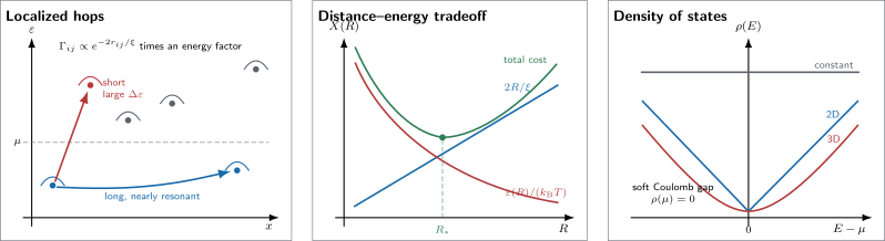
Hopping transport balances overlap and energy matching. A short hop can require a large activation energy, whereas a longer hop can find a nearly resonant state. Their sum has an optimum $R_\ast$. A constant density of states produces Mott exponents; long-range interactions suppress the density of states near $\mu$, producing linear and quadratic Coulomb gaps in two and three dimensions.

Optimal distance and energy

At scaling accuracy,

$$\frac{R_\ast}{\xi} \sim \left( \frac{T_{\mathrm M}}{T} \right)^{1/(d+1)}$$

and

$$\frac{\varepsilon_\ast}{k_{\mathrm B}T} \sim \left( \frac{T_{\mathrm M}}{T} \right)^{1/(d+1)}.$$

Cooling therefore lengthens the typical hop while narrowing its energy window. The phrase “variable range” refers to this temperature-dependent spatial optimization.

The derivation requires:

$$R_\ast\gg\xi, \qquad \varepsilon_\ast \ \text{inside a constant-DOS window},$$

and a sufficiently large sample. Linear response additionally requires the field work over an optimal hop to be small:

$$eER_\ast \ll k_{\mathrm B}T$$

at the level of the standard rate model. When this condition fails, field-assisted hopping and electron heating can mimic a different temperature exponent.

Crossovers

A single sample can pass through several regimes:

$$\text{activation} \longrightarrow \text{Mott VRH} \longrightarrow \text{interaction-modified VRH}$$

as temperature is lowered. The sequence is not automatic. A finite sample can saturate when $R_\ast$ reaches a device dimension; a nearby gate can screen interactions; a changing dielectric constant can shift $T_0$; and electron–phonon decoupling can replace the electron temperature by a bias-dependent value.

Interactions and the Coulomb Gap

Stability of localized charges

For localized electrons with long-range repulsion, a schematic site Hamiltonian is

$$\begin{aligned} H ={}& \sum_i \varepsilon_i^{(0)}n_i \\ &+ \frac12 \sum_{i\ne j} \frac{ e^2 }{ 4\pi\epsilon_0\kappa r_{ij} } \left( n_i-\bar n_i \right) \left( n_j-\bar n_j \right). \end{aligned}$$

Let $\widetilde\varepsilon_i<0$ be the interaction-renormalized energy of an occupied site and $\widetilde\varepsilon_j>0$ that of an empty site, measured from $\mu$. Moving the electron from $i$ to $j$ costs

$$\Delta E_{ij} = \widetilde\varepsilon_j -\widetilde\varepsilon_i - \frac{ e^2 }{ 4\pi\epsilon_0\kappa r_{ij} }.$$

The final term is the attraction between the created electron and hole. Stability of the ground state requires

$$\Delta E_{ij}>0$$

for every occupied–empty pair. Two sites extremely close to the chemical potential therefore cannot also be arbitrarily close in space.

Soft density-of-states suppression

Let $n(\varepsilon)$ be the concentration of sites within energy $\varepsilon$ of $\mu$. Their typical spacing is

$$r(\varepsilon) \sim \left[ n(\varepsilon) \right]^{-1/d}.$$

The stability inequality implies, at scaling accuracy,

$$\varepsilon \gtrsim \frac{ e^2 }{ 4\pi\epsilon_0\kappa r(\varepsilon) }.$$

Hence

$$n(\varepsilon) \lesssim \left( \frac{ 4\pi\epsilon_0\kappa\varepsilon }{ e^2 } \right)^d,$$

and differentiating with respect to energy gives the stability bound

$$\rho(E) \lesssim A_d \left( \frac{ 4\pi\epsilon_0\kappa }{ e^2 } \right)^d \lvert E-\mu\rvert^{d-1},$$

where $A_d$ is a geometry-dependent constant. The self-consistent Efros–Shklovskii solution saturates this power-law bound at scaling accuracy for the standard unscreened case in $d>1$. Thus,

$$\begin{aligned} \rho_{2\mathrm D}(E) &\propto \lvert E-\mu\rvert, \\ \rho_{3\mathrm D}(E) &\propto \lvert E-\mu\rvert^2. \end{aligned}$$

This is a soft gap: the density of states vanishes at one energy but is nonzero arbitrarily nearby. It is not a hard band gap, a superconducting gap, or the charging gap of one isolated island. Finite temperature, finite size, metallic screening, and nonequilibrium occupations round the ideal asymptote.

Efros–Shklovskii hopping

More generally, suppose

$$\rho(E) \propto \lvert E-\mu\rvert^s.$$

Counting available sites gives

$$R^d\varepsilon^{s+1} \sim \text{constant}.$$

Optimizing the distance and energy costs then yields

$$p = \frac{ s+1 }{ s+d+1 }.$$

For a Coulomb gap, $s=d-1$, so

$$p_{\mathrm{ES}} = \frac12$$

in both two and three dimensions. The conductivity becomes

$$\sigma(T) = \sigma_{\mathrm{ES}}(T) \exp \left[ -\left( \frac{T_{\mathrm{ES}}}{T} \right)^{1/2} \right],$$

where

$$T_{\mathrm{ES}} = C_{\mathrm{ES}} \frac{ e^2 }{ 4\pi\epsilon_0\kappa k_{\mathrm B}\xi }.$$

The numerical constant $C_{\mathrm{ES}}$ is network- and convention-dependent. Unlike $T_{\mathrm M}$, the leading Efros–Shklovskii scale depends directly on dielectric screening and $\xi$, not on a constant $\rho_0$ that the Coulomb gap has already invalidated.

Screening and interaction limits

A metallic gate, large polarizability, mobile carriers, or finite screening length cuts off the $1/r$ interaction. At energies below the corresponding screening scale, the Coulomb gap can fill or change form and Mott-like hopping may re-emerge. A fit that assigns $p=1/2$ while ignoring a gate closer than the inferred hopping length is physically incomplete.

Interactions can also produce glassy relaxation, occupation correlations, multiparticle hops, and history dependence. Those phenomena motivate the term electron glass, but slow relaxation is not required by the definition of a noninteracting Anderson insulator. Many-Body Localization Preview treats the distinct question of memory and entanglement in an isolated interacting quantum system.

Identifying the Transport Law

Reduced activation energy

Several stretched exponentials can look nearly linear over a narrow plotting window. For

$$R(T) = R_0 \exp \left[ \left( \frac{T_0}{T} \right)^p \right],$$

define

$$W(T) \equiv - \frac{d\ln R}{d\ln T}.$$

If the prefactor is constant,

$$W(T) = p \left( \frac{T_0}{T} \right)^p$$

and

$$\frac{d\ln W}{d\ln T} = -p.$$

A log–log plot of $W$ can therefore estimate $p$ without choosing in advance among $T^{-1}$, $T^{-1/2}$, $T^{-1/3}$, and $T^{-1/4}$ axes. Numerical differentiation amplifies noise, and a prefactor

$$\sigma_0(T)\propto T^m$$

adds a competing contribution. Derivative smoothing, uncertainty propagation, and fit-window stability must be reported.

Parameter closure

A transport exponent is strongest when its scale closes against independent information:

Candidate law	Fitted scale	Independent closure
Activation	$E_a=k_{\mathrm B}T_a$	Spectral gap, mobility-edge offset, or known barrier
Mott VRH	$T_{\mathrm M}\propto[\rho_0\xi^d]^{-1}$	Tunneling DOS or thermodynamic DOS plus localization length
Efros–Shklovskii VRH	$T_{\mathrm{ES}}\propto(\kappa\xi)^{-1}$	Dielectric response plus localization length
Finite-size saturation	$R_\ast(T)\sim L$	Device dimensions and geometry dependence
Non-Ohmic hopping	$eER_\ast\sim k_{\mathrm B}T$	Bias dependence and electron-temperature control

Magnetoresistance can provide additional evidence, but hopping magnetoresistance has several competing mechanisms: wavefunction shrinkage, interference among alternative paths, spin blockade, and field-dependent density of states. Its sign is not a unique label.

Evidence ladder

1. Suggestive: resistance rises on cooling.
2. Model-like: one stretched exponential fits a declared range.
3. Discriminating: derivative and residual tests separate competing exponents and prefactors.
4. Parameter-closed: $T_0$, $\xi$, $\rho_0$, $\kappa$, and dimensionality agree quantitatively.
5. Mechanism-level: spectroscopy, size scaling, field dependence, and heating controls support localized states and the proposed bath-assisted network.

Common Mistakes

• Equating finite density of states with metallic transport.
• Calling an Anderson insulator “gapped” without specifying a mobility gap rather than a spectral gap.
• Deriving finite-temperature hopping from a closed static one-particle Hamiltonian without an energy-exchange mechanism.
• Using an overlap amplitude $\exp(-r/\xi)$ where a rate requires its square, $\exp(-2r/\xi)$.
• Averaging pair resistances instead of finding the critical percolating network.
• Treating $p=1/(d+1)$ as valid when the active density of states is not constant.
• Calling every $p=1/2$ fit Efros–Shklovskii hopping; ordinary one-dimensional Mott scaling and other mechanisms can share that exponent.
• Ignoring a temperature-dependent prefactor when extracting $p$.
• Fitting three decades of resistance that span only a small range of $T^{-p}$ and declaring a unique law by eye.
• Inferring $\xi$ from $T_{\mathrm{ES}}$ without an independently justified dielectric constant and numerical convention.
• Ignoring contacts, leakage, finite-size saturation, electron heating, and non-Ohmic bias.
• Confusing a Coulomb gap with Coulomb blockade in a fabricated island.
• Treating interaction-modified hopping transport as evidence for many-body localization.

Exercises

1. Finite density of states, zero conductivity

An idealized localized system has

$$\rho(E_{\mathrm F}) = 2.0\times10^{46} \ \mathrm{J^{-1}m^{-3}}, \qquad D(E_{\mathrm F})=0.$$

What does the Einstein relation predict, and which part of the input distinguishes this system from a band insulator?

Solution

The Einstein relation gives

$$\sigma = e^2\rho(E_{\mathrm F})D(E_{\mathrm F}) = 0.$$

The nonzero density of states distinguishes it from an ideal hard-gap band insulator, for which $\rho(E_{\mathrm F})=0$. Here states exist but do not diffuse.

2. Detailed balance for a hop

Let $\varepsilon_j-\varepsilon_i=\Delta>0$. Use the Miller–Abrahams rates to show detailed balance between $i$ and $j$.

Solution

The uphill rate is

$$\Gamma_{i\to j} = \Gamma_0 e^{-2r_{ij}/\xi} e^{-\Delta/(k_{\mathrm B}T)}.$$

The reverse hop is downhill:

$$\Gamma_{j\to i} = \Gamma_0 e^{-2r_{ij}/\xi}.$$

Therefore

$$\frac{\Gamma_{i\to j}}{\Gamma_{j\to i}} = e^{-\Delta/(k_{\mathrm B}T)},$$

which is the required Boltzmann ratio.

3. Derive the Mott exponent

Starting from

$$X(R) = \frac{2R}{\xi} + \frac{1}{\rho_0k_{\mathrm B}TR^d},$$

derive the temperature exponent in the conductivity.

Solution

The stationary condition is

$$\frac{2}{\xi} = \frac{d}{ \rho_0k_{\mathrm B}TR_\ast^{d+1} }.$$

Thus

$$R_\ast \propto T^{-1/(d+1)}.$$

At the optimum, the energy term is proportional to the distance term, so

$$X(R_\ast) \propto \frac{R_\ast}{\xi} \propto T^{-1/(d+1)}.$$

Since $\sigma\propto e^{-X}$,

$$\sigma \propto \exp \left[ -\left( \frac{T_{\mathrm M}}{T} \right)^{1/(d+1)} \right].$$

4. Optimal-hop scale in two dimensions

Use the scaling forms

$$\frac{R_\ast}{\xi} \simeq \left( \frac{T_{\mathrm M}}{T} \right)^{1/3}, \qquad X_\ast \simeq \left( \frac{T_{\mathrm M}}{T} \right)^{1/3}.$$

For $T_{\mathrm M}=900\ \mathrm K$ and $T=4.0\ \mathrm K$, estimate $R_\ast/\xi$ and $e^{X_\ast}$.

Solution

The ratio is

$$\frac{T_{\mathrm M}}{T} = 225.$$

Therefore

$$\frac{R_\ast}{\xi} \simeq 225^{1/3} \simeq 6.08.$$

The exponential resistance factor is

$$e^{X_\ast} \simeq e^{6.08} \simeq 4.4\times10^2.$$

The numerical prefactors are illustrative; a percolation calculation changes order-one constants.

5. A general soft-gap exponent

Suppose $\rho(E)\propto\lvert E-\mu\rvert^s$. Derive

$$p = \frac{s+1}{s+d+1}.$$

Then evaluate it for a Coulomb gap.

Solution

The number of sites within radius $R$ and energy width $\varepsilon$ scales as

$$\mathcal N \sim R^d\varepsilon^{s+1}.$$

Setting $\mathcal N\sim1$ gives

$$\varepsilon(R) \propto R^{-d/(s+1)}.$$

The hopping exponent has the form

$$X(R) \sim R + \frac{ R^{-d/(s+1)} }{ T },$$

with fixed microscopic factors suppressed. Minimization gives

$$R_\ast \propto T^{-(s+1)/(s+d+1)}.$$

Both optimized costs have that temperature power, so

$$p = \frac{s+1}{s+d+1}.$$

For an unscreened Coulomb gap, $s=d-1$, hence

$$p = \frac{d}{2d} = \frac12.$$

6. Efros–Shklovskii temperature

Take $\kappa=12$, $\xi=10\ \mathrm{nm}$, and $C_{\mathrm{ES}}=2.8$. Use

$$\frac{e^2}{4\pi\epsilon_0} \simeq 1.440\ \mathrm{eV\,nm}$$

to estimate $T_{\mathrm{ES}}$. Then find the hopping exponent at $T=4.0\ \mathrm K$.

Solution

The interaction energy at $\xi$ is

$$\frac{ e^2 }{ 4\pi\epsilon_0\kappa\xi } = \frac{ 1.440\ \mathrm{eV\,nm} }{ 12\times10\ \mathrm{nm} } = 0.0120\ \mathrm{eV}.$$

Using $1\ \mathrm{eV}/k_{\mathrm B}\simeq11604.5\ \mathrm K$,

$$T_{\mathrm{ES}} \simeq 2.8\times0.0120\times11604.5\ \mathrm K \simeq 390\ \mathrm K.$$

At $4.0\ \mathrm K$,

$$\left( \frac{T_{\mathrm{ES}}}{T} \right)^{1/2} \simeq \left( \frac{390}{4.0} \right)^{1/2} \simeq 9.87.$$

7. Reduced activation-energy slopes

What slope should a plot of $\ln W$ against $\ln T$ have for Arrhenius, two-dimensional Mott, three-dimensional Mott, and Efros–Shklovskii transport?

Solution

For a constant prefactor,

$$\frac{d\ln W}{d\ln T} = -p.$$

Therefore:

$$\begin{array}{l|c} \text{law}&\text{slope}\\ \hline \text{Arrhenius}&-1\\ \text{2D Mott}&-1/3\\ \text{3D Mott}&-1/4\\ \text{Efros–Shklovskii}&-1/2 \end{array}$$

A temperature-dependent prefactor or crossover makes the slope drift rather than remain constant.

8. Audit a hopping claim

A two-dimensional gated film fits $R\propto\exp[(T_0/T)^{1/2}]$ from $2$ to $8\ \mathrm K$. The authors call this proof of an Efros–Shklovskii Coulomb gap. List at least seven further checks.

Solution

A strong audit should ask for:

1. comparison with Arrhenius, $p=1/3$, and free-$p$ fits using residuals rather than visual linearity;
2. reduced activation-energy analysis and treatment of the prefactor;
3. confirmation that voltage bias is Ohmic and electron heating is negligible;
4. independent estimates of $\kappa$ and $\xi$ that reproduce $T_0$;
5. evidence that the inferred optimal hopping length is below sample dimensions;
6. comparison of that length with gate distance and screening length;
7. tunneling or compressibility evidence for a soft density-of-states suppression;
8. contact and leakage controls, preferably including four-terminal data;
9. stability across temperature windows and devices;
10. exclusion of one-dimensional bottlenecks, granular charging, and magnetic mechanisms.

The fitted exponent is compatible with Efros–Shklovskii transport, but it is not unique proof by itself.

Connections

• Metals, Insulators, and Semiconductors compares band, Mott, Anderson, and topological insulating mechanisms.
• Anderson Localization owns localized eigenfunctions, localization length, transfer matrices, mobility-edge basics, and direct diagnostics.
• Scaling Theory of Localization develops the zero-temperature coherent conductance flow into the localized regime.
• Mobility Edges distinguishes activation into extended states from hopping within localized states and owns the energy-resolved critical boundary.
• Disorder in Quantum Matter defines quenched disorder ensembles, scattering lengths, and the distinction between static disorder and dynamic noise.
• Quantum Coherence in Conductors distinguishes elastic localization physics from dephasing and environmental energy exchange.
• Coulomb Blockade separates a soft Coulomb gap in a distributed localized system from the charging energy of a discrete island.
• Drude Theory supplies the extended-state transport baseline that hopping replaces.
• Spectral Functions distinguishes density of states, linewidth, quasiparticle weight, and transport lifetime.
• Many-Body Localization Preview separates bath-assisted hopping in a localized solid from isolated interacting dynamics and entanglement memory.
• One-over-f Noise treats broad fluctuator ensembles that can accompany glassy hopping systems without defining the Anderson insulator itself.

References

1. P. W. Anderson, “Absence of Diffusion in Certain Random Lattices,” Physical Review 109, 1492–1505 (1958), doi:10.1103/PhysRev.109.1492. Establishes localization by static disorder without requiring a spectral gap.
2. A. Miller and E. Abrahams, “Impurity Conduction at Low Concentrations,” Physical Review 120, 745–755 (1960), doi:10.1103/PhysRev.120.745. Derives phonon-assisted localized-site rates and the equivalent resistor network.
3. N. F. Mott, “Conduction in Glasses Containing Transition Metal Ions,” Journal of Non-Crystalline Solids 1, 1–17 (1968), doi:10.1016/0022-3093(68)90002-1. Develops the distance–energy optimization behind variable-range hopping.
4. V. Ambegaokar, B. I. Halperin, and J. S. Langer, “Hopping Conductivity in Disordered Systems,” Physical Review B 4, 2612–2620 (1971), doi:10.1103/PhysRevB.4.2612. Formulates the critical-path and percolation treatment of the hopping network.
5. A. L. Efros and B. I. Shklovskii, “Coulomb Gap and Low Temperature Conductivity of Disordered Systems,” Journal of Physics C: Solid State Physics 8, L49–L51 (1975), doi:10.1088/0022-3719/8/4/003. Derives the soft interaction gap and the $p=1/2$ hopping law.
6. P. A. Lee and T. V. Ramakrishnan, “Disordered Electronic Systems,” Reviews of Modern Physics 57, 287–337 (1985), doi:10.1103/RevModPhys.57.287. Reviews localization, interactions, and insulating transport.
7. R. Rosenbaum, “Crossover from Mott to Efros–Shklovskii Variable-Range-Hopping Conductivity in Amorphous In-O Films,” Physical Review B 44, 3599–3603 (1991), doi:10.1103/PhysRevB.44.3599. Reports and audits a Mott-to-Coulomb-gap crossover.
8. M. E. Raikh, J. Czingon, Q. Ye, F. Koch, W. Schoepe, and K. Ploog, “Mechanisms of Magnetoresistance in Variable-Range-Hopping Transport for Two-Dimensional Electron Systems,” Physical Review B 45, 6015–6025 (1992), doi:10.1103/PhysRevB.45.6015. Demonstrates the nonuniqueness of hopping magnetoresistance mechanisms.
9. M. Lee, J. G. Massey, V. L. Nguyen, and B. I. Shklovskii, “Coulomb Gap in a Doped Semiconductor near the Metal-Insulator Transition,” Physical Review B 60, 1582–1591 (1999), doi:10.1103/PhysRevB.60.1582. Uses tunneling spectroscopy to probe the interaction-modified density of states.
10. V. Y. Butko, J. F. DiTusa, and P. W. Adams, “Coulomb Gap: How a Metal Film Becomes an Insulator,” Physical Review Letters 84, 1543–1546 (2000), doi:10.1103/PhysRevLett.84.1543. Tracks a tunneling zero-bias anomaly into a nonperturbative Coulomb gap.
11. T. G. Castner, “Variable-Range Hopping in the Critical Regime,” Physical Review B 61, 16596–16605 (2000), doi:10.1103/PhysRevB.61.16596. Shows how critical dielectric and localization scales modify textbook hopping laws.
12. D. Joung and S. I. Khondaker, “Efros–Shklovskii Variable-Range Hopping in Reduced Graphene Oxide Sheets of Varying Carbon Fraction,” Physical Review B 86, 235423 (2012), doi:10.1103/PhysRevB.86.235423. Combines low-field temperature scaling with field-driven transport and inferred localization lengths.
13. N. Papadopoulos, G. A. Steele, and H. S. J. van der Zant, “Efros–Shklovskii Variable Range Hopping and Nonlinear Transport in 1T/1T′-MoS2,” Physical Review B 96, 235436 (2017), doi:10.1103/PhysRevB.96.235436. Demonstrates contact, Ohmic, nonlinear-field, and parameter-closure checks in a two-dimensional material.
14. O. Asban, A. Burin, A. Shnirman, and M. Schechter, “Polaronic Effect of a Metal Layer on Variable Range Hopping,” Physical Review B 103, 045129 (2021), doi:10.1103/PhysRevB.103.045129. Separates static screening of the Coulomb gap from dynamical environmental effects.

Further Reading

• N. F. Mott and E. A. Davis, Electronic Processes in Non-Crystalline Materials, 2nd ed., Oxford University Press, 1979. A classic treatment of impurity bands, hopping, and amorphous transport.
• B. I. Shklovskii and A. L. Efros, Electronic Properties of Doped Semiconductors, Springer, 1984. The standard monograph on hopping networks, Coulomb gaps, and metal–insulator transitions.
• A. L. Efros and M. Pollak, eds., Electron–Electron Interactions in Disordered Systems, North-Holland, 1985. Advanced treatments of interaction corrections and Coulomb-glass physics.