Glasses and Spin Glasses

A glass is a disordered state with relaxation times so broad and long that observation depends on preparation and waiting history; a spin glass is a magnetic realization in which competing interactions freeze random local spin orientations without ordinary uniform or staggered order. Slow dynamics alone is not a complete phase definition. A rigorous claim must separate equilibrium order, finite-time freezing, metastability, and instrumental blocking.

This page is the canonical home for quenched frustration in spin models, Edwards–Anderson overlap order, the Sherrington–Kirkpatrick benchmark, replica ideas, aging, memory, and the bridge to structural and quantum glasses. Disorder in Quantum Matter owns random-variable ensembles, quenched versus annealed averaging, and microscopic disorder audits. Order Parameters owns the general source-selected thermodynamic definition. Relaxation and Thermalization owns generic equilibration, dephasing, and ensemble identification.

The defining caution is:

$$\begin{gathered} \text{slow or history-dependent response} \\ \not\Longrightarrow \\ \text{equilibrium spin-glass phase} \end{gathered}$$

without scaling, time-window, and competing-mechanism tests.

Convention and Status Ledger

Item	Convention or status on this page	Consequence
Classical spins	$S_i=\pm1$ unless a vector or quantum model is declared	Signs in the bond Hamiltonian remain unambiguous
Bond convention	$H=-\sum_{ij}J_{ij}S_iS_j$	$J_{ij}>0$ favors alignment
Disorder average	$[X]_J$	It is distinct from the thermal average $\langle X\rangle_J$
Replica	Independent equilibrium copy with the same bonds	It is not an additional physical sample
Finite system	Global spin-flip symmetry is unbroken at zero field	Naive $\langle S_i\rangle_J^2$ vanishes
SK thermodynamics	Parisi variational free energy is mathematically established	The result is specific to a mean-field model class
3D short-range order	A finite-temperature Ising spin-glass transition is strongly supported numerically	The detailed low-temperature pure-state structure remains disputed
Field stability	The SK de Almeida–Thouless line is standard mean-field physics	A corresponding line in realistic short-range systems is unsettled
Structural glass	No quenched random bonds are required	Spin-glass language is a bridge, not an exact identification
Effective temperature	Used only after observable and timescale checks	A fitted fluctuation–dissipation ratio is not automatically thermodynamic

The page therefore mixes standard definitions with active research. Each frontier statement is labeled by model and dimension.

Frustration and Randomness

Two ingredients that are not equivalent

Frustration means that locally preferred constraints cannot all be satisfied in one configuration. Randomness means that couplings, fields, positions, or occupancies vary across the sample. Neither implies the other.

• A triangular antiferromagnet is frustrated without quenched randomness and can still order.
• A ferromagnet with random positive bonds is disordered but unfrustrated.
• A structural glass can develop glassy dynamics without externally imposed random couplings.
• A canonical metallic spin glass combines random magnetic positions with sign-changing RKKY interactions.

Antiferromagnetism owns geometric frustration and ordered $120^\circ$ states. RKKY Interaction derives the oscillatory exchange that frustrates dilute metallic moments.

Loop criterion for Ising bonds

Consider

$$H_J = - \sum_{\langle i,j\rangle} J_{ij}S_iS_j.$$

A local gauge transformation

$$S_i \longmapsto \eta_iS_i, \qquad \eta_i=\pm1,$$

accompanied by

$$J_{ij} \longmapsto \eta_i\eta_jJ_{ij}$$

leaves the energy unchanged. The sign product around a closed loop $C$,

$$\Phi_C = \prod_{(ij)\in C} \operatorname{sgn}(J_{ij}),$$

is gauge invariant. If

$$\Phi_C=-1,$$

the loop contains an odd number of antiferromagnetic signs and at least one bond must be unsatisfied. This criterion is exact for Ising pair constraints. Vector spins, multi-spin interactions, random fields, and quantum terms require broader notions of frustration.

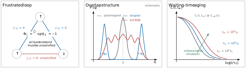
Three layers of a spin-glass claim. Left: the gauge-invariant sign product $\Phi_\triangle=-1$ forces at least one unsatisfied Ising bond. Center: the overlap distribution distinguishes a paramagnet from low-temperature alternatives; the two-peak droplet and broad replica-symmetry-breaking curves are schematic competing scenarios, not interchangeable fits. Right: after a quench, the correlation $C(t,t_w)$ depends on waiting time $t_w$, violating equilibrium time-translation invariance.

Edwards–Anderson model

The short-range benchmark is

$$H_{\mathrm{EA}} = - \sum_{\langle i,j\rangle} J_{ij}S_iS_j - h \sum_iS_i.$$

Typical choices are Gaussian bonds,

$$[J_{ij}]_J = 0, \qquad [J_{ij}^2]_J = J^2,$$

or binary bonds $J_{ij}=\pm J$. The lattice, dimension, boundary conditions, field, and bond distribution are part of the model. Universality can make some critical exponents insensitive to microscopic details, but it does not make finite-size data or transition temperatures convention-free.

For a fixed realization $J$, the partition function is

$$Z_J = \sum_{\{S_i\}} e^{-\beta H_J}.$$

The quenched free energy is

$$F_{\mathrm q} = - k_{\mathrm B}T [\ln Z_J]_J,$$

whereas annealed disorder would give

$$F_{\mathrm a} = - k_{\mathrm B}T \ln[Z_J]_J.$$

Concavity of the logarithm implies

$$F_{\mathrm q} \geq F_{\mathrm a}.$$

In a magnetic alloy the impurity arrangement is ordinarily frozen on the spin-relaxation timescale, so the quenched average is the relevant one.

Rugged landscapes and metastability

For one realization, define the energy of a configuration $\mathbf S$ by $E_J(\mathbf S)$. Frustration produces many local minima separated by barriers. A minimum relative to single-spin flips need not be stable to collective rearrangements, and the number of minima depends on the chosen move set.

A metastable state is also not automatically a thermodynamic pure state. Metastability is dynamical and time-window dependent; a pure state is an infinite-volume equilibrium concept. Confusing the two turns an optimization landscape into an unsupported phase diagram.

Spin-Glass Order

Frozen local moments without ordinary magnetization

The uniform magnetization is

$$m = \frac{1}{N} \sum_i [\langle S_i\rangle_J]_J.$$

It vanishes in a zero-field spin glass after disorder averaging. The Edwards–Anderson order parameter instead measures the squared local frozen expectation in a selected pure state $\alpha$:

$$q_{\mathrm{EA}} = \frac{1}{N} \sum_i \left[ \langle S_i\rangle_{\alpha,J}^2 \right]_J.$$

The square is taken before the disorder average, so random signs do not cancel. At zero field, a finite Gibbs state respects global spin flip and has

$$\langle S_i\rangle_J = 0.$$

One must select a pure state with an infinitesimal source or use correlation and replica diagnostics before taking the thermodynamic limit. The order of operations is physical:

$$\lim_{h\to0^+} \lim_{N\to\infty} \neq \lim_{N\to\infty} \lim_{h\to0}.$$

A dynamical equilibrium definition is

$$q_{\mathrm{EA}} = \lim_{t\to\infty} \lim_{N\to\infty} \frac{1}{N} \sum_i \left[ \langle S_i(t)S_i(0) \rangle_J \right]_J,$$

with the equilibrium state and order of limits declared. In a laboratory that falls out of equilibrium, a finite observation-time plateau is evidence of freezing, not automatically the infinite-time value.

Two replicas and the overlap

Take two independent equilibrium configurations, $S^{(1)}$ and $S^{(2)}$, subject to the same bond realization. Their spin overlap is

$$q_{12} = \frac{1}{N} \sum_i S_i^{(1)}S_i^{(2)}.$$

For one sample,

$$P_J(q) = \left\langle \delta(q-q_{12}) \right\rangle_J,$$

and the disorder-averaged distribution is

$$P(q) = [P_J(q)]_J.$$

At zero field and finite size, $P_J(q)$ is symmetric under $q\to-q$. A high-temperature paramagnet narrows toward $q=0$. A low-temperature glass develops nonzero overlap weight, but its thermodynamic shape is model dependent.

Scenario	Idealized thermodynamic overlap structure	Status
SK full replica symmetry breaking	broad hierarchy of overlaps	established for the mean-field model
Droplet or scaling picture	one symmetry-related pair of pure states; weight at $\pm q_{\mathrm{EA}}$	viable short-range scenario
Chaotic-pairs or metastate pictures	sample-size-dependent state pair selected from many possibilities	active short-range framework
Finite simulation	rounded, sample-dependent peaks and central weight	cannot identify a scenario without scaling

The overlap is not a conventional local observable in one replica, but it is operational in simulations and in coupled-copy protocols.

Spin-glass susceptibility and correlation length

At zero field, the spin-glass susceptibility is

$$\chi_{\mathrm{SG}} = \frac{1}{N} \sum_{i,j} \left[ \langle S_iS_j\rangle_J^2 \right]_J.$$

For two independent replicas with common disorder,

$$\chi_{\mathrm{SG}} = N \left[ \langle q_{12}^2\rangle_J \right]_J.$$

In a field, use connected correlations:

$$\chi_{\mathrm{SG}}^{\mathrm c} = \frac{1}{N} \sum_{i,j} \left[ \left( \langle S_iS_j\rangle_J - \langle S_i\rangle_J \langle S_j\rangle_J \right)^2 \right]_J.$$

Define the spatial glass correlator

$$G_{\mathrm{SG}}(\mathbf r) = \frac{1}{N} \sum_i \left[ \langle S_iS_{i+\mathbf r} \rangle_J^2 \right]_J$$

at zero field, and let $\widetilde G_{\mathrm{SG}}(\mathbf k)$ be its Fourier transform. A common second-moment finite-size length is

$$\xi_L = \frac{1}{ 2\sin(k_{\min}/2) } \left[ \frac{ \widetilde G_{\mathrm{SG}}(\mathbf 0) }{ \widetilde G_{\mathrm{SG}}(\mathbf k_{\min}) } - 1 \right]^{1/2}.$$

Crossings of $\xi_L/L$ across several sizes are far stronger evidence for a thermodynamic transition than a single broad peak in susceptibility. Covariance, corrections to scaling, equilibration, and disorder tails must still be audited.

Experimental evidence ladder

Canonical signatures include:

1. a low-field ac-susceptibility cusp whose apparent freezing temperature shifts with frequency;
2. divergence or strong growth of the nonlinear susceptibility under controlled field and frequency limits;
3. separation of field-cooled and zero-field-cooled protocols;
4. remanence and slow logarithmic or broad-spectrum relaxation;
5. waiting-time aging, memory, and rejuvenation;
6. local-probe evidence for frozen random moments without magnetic Bragg order;
7. scaling against frequency, field, sample size, and observation time.

A superparamagnetic assembly, cluster glass, blocked nanoparticles, domain-wall system, or chemically inhomogeneous magnet can reproduce several items. A mature claim combines thermodynamic scaling with local structure and explicit blocking controls.

The characteristic time is often fitted either to critical slowing,

$$\tau = \tau_0 \left| \frac{ T_f-T_g }{ T_g } \right|^{-z\nu},$$

or to a Vogel–Fulcher form,

$$\tau = \tau_0 \exp\!\left[ \frac{A}{ T_f-T_0 } \right].$$

Over a narrow frequency interval, both can fit. The inferred $\tau_0$, $T_g$ or $T_0$, exponent, residuals, and stability to the fit window are part of the evidence.

Sherrington–Kirkpatrick Mean-Field Benchmark

The infinite-range Ising model is

$$H_{\mathrm{SK}} = - \sum_{i<j} J_{ij}S_iS_j - h \sum_iS_i,$$

with

$$[J_{ij}]_J = \frac{J_0}{N}, \qquad \left[ \left( J_{ij} - \frac{J_0}{N} \right)^2 \right]_J = \frac{J^2}{N}.$$

The $N^{-1/2}$ width keeps the random interaction energy extensive. Setting $J_0=0$ isolates the spin-glass instability.

In the replica-symmetric approximation at zero field, the overlap satisfies

$$q = \int_{-\infty}^{\infty} Dz\, \tanh^2\!\left( \beta J\sqrt q\,z \right),$$

where

$$Dz = \frac{ e^{-z^2/2} }{ \sqrt{2\pi} } dz.$$

Linearizing at small $q$ gives

$$q \simeq (\beta J)^2q,$$

and therefore

$$k_{\mathrm B}T_c = J.$$

The replica-symmetric free-energy density is

$$\begin{aligned} f_{\mathrm{RS}} &= - \frac{\beta J^2}{4} (1-q)^2 \\ &\quad - \frac{1}{\beta} \int Dz\, \ln\!\left[ 2\cosh( \beta J\sqrt q\,z+\beta h ) \right]. \end{aligned}$$

Its local stability is controlled by the replicon eigenvalue

$$\lambda_{\mathrm R} = 1 - (\beta J)^2 \int Dz\, \operatorname{sech}^4\!\left( \beta J\sqrt q\,z+\beta h \right).$$

The de Almeida–Thouless boundary satisfies

$$\lambda_{\mathrm R} = 0.$$

Below that line the replica-symmetric saddle is unstable and the Parisi hierarchy is required. This result is exact within the SK mean-field setting; it does not establish a field-stable glass phase in every short-range magnet.

Replica Ideas Preview

The quenched logarithm

The obstacle is the disorder average of $\ln Z_J$. For positive integer $n$,

$$Z_J^n = \prod_{a=1}^{n} \sum_{\{S_i^a\}} e^{-\beta H_J[S^a]},$$

which introduces $n$ copies sharing the same disorder. The formal identity is

$$[\ln Z_J]_J = \lim_{n\to0} \frac{ [Z_J^n]_J-1 }{ n }.$$

The procedure is:

1. compute $[Z_J^n]_J$ for positive integer $n$;
2. express the answer in terms of replica overlaps;
3. analytically continue away from integer $n$;
4. take $n\to0$.

Step 3 is the delicate one. Values at positive integers do not by themselves determine a unique analytic continuation. The replica trick, or replica method, is a powerful formal calculus whose predictions must be checked against controlled solutions, rigorous methods, or independent numerics.

Overlap matrix

Disorder averaging couples replicas through

$$q_{ab} = \frac{1}{N} \sum_i S_i^aS_i^b, \qquad a\neq b.$$

A replica-symmetric ansatz sets

$$q_{ab} = q$$

for every $a\neq b$. The low-temperature SK saddle violates this permutation symmetry in a hierarchical way. In the full Parisi construction, the discrete hierarchy becomes a function

$$q(x), \qquad 0\leq x\leq1,$$

related to the distribution of overlaps among equilibrium states. Replica symmetry breaking is therefore more than “many local minima”: it is a specific organization of equilibrium Gibbs weight.

What is established and what is not

The Parisi variational formula gives the exact thermodynamic free energy of the SK model. Guerra established the matching variational bound needed for the program, and Talagrand proved the formula. These results vindicate a central mean-field prediction without turning every formal $n\to0$ manipulation into a general theorem.

For the three-dimensional short-range Edwards–Anderson model:

• numerical work strongly supports a finite-temperature zero-field transition for Ising spins;
• the number and organization of low-temperature pure states remain debated;
• droplet, replica-symmetry-breaking, chaotic-pairs, and related metastate descriptions make different thermodynamic predictions;
• the existence of a de Almeida–Thouless-like line in a field is not settled.

A page that presents the SK overlap hierarchy as an established description of all laboratory spin glasses would overstate the evidence.

Aging and Slow Dynamics

Waiting-time protocol

Quench the system from high temperature to a low measuring temperature, wait for time $t_w$, and then observe for an additional lag $t$. Define

$$C(t,t_w) = \frac{1}{N} \sum_i \left[ \left\langle S_i(t_w+t) S_i(t_w) \right\rangle \right]_J.$$

In equilibrium, time-translation invariance gives

$$C(t,t_w) = C_{\mathrm{eq}}(t).$$

In an aging system,

$$\frac{\partial C(t,t_w)}{ \partial t_w } \neq 0.$$

Older samples commonly decorrelate more slowly. A useful decomposition is

$$C(t,t_w) \simeq C_{\mathrm{st}}(t) + C_{\mathrm{ag}} \!\left( \frac{ h(t_w+t) }{ h(t_w) } \right),$$

where $h$ is a model- and protocol-dependent clock. Simple $t/t_w$ aging is not universal; subaging and multiple sectors are common.

Response and fluctuation–dissipation ratio

Let

$$R(t,s) = \frac{1}{N} \sum_i \left. \frac{ \delta \langle S_i(t)\rangle }{ \delta h_i(s) } \right|_{h=0}$$

for $t>s$. At equilibrium, the classical fluctuation–dissipation theorem gives

$$k_{\mathrm B}T R(t,s) = \frac{ \partial C(t,s) }{ \partial s }.$$

Out of equilibrium, define

$$k_{\mathrm B}T R(t,s) = X(t,s) \frac{ \partial C(t,s) }{ \partial s }.$$

Fast quasi-equilibrated modes often have $X\simeq1$, while slow aging sectors can have $X\neq1$. An effective temperature

$$T_{\mathrm{eff}} = \frac{T}{X}$$

is meaningful only if the long-time ratio is stable, observable independent within a sector, and consistent with a weak thermometer. A curved response–correlation plot or frequency-dependent $X$ is not one scalar temperature.

Fluctuation–Dissipation Relation owns the equilibrium theorem, quantum ordering conventions, and bath assumptions. Here its violation is used as a nonequilibrium glass diagnostic.

Memory and rejuvenation

In a temperature-stop protocol:

1. cool to $T_1<T_g$ and wait;
2. cool further to $T_2$;
3. reheat through $T_1$.

The response can resume aging at $T_2$ as though newly prepared, called rejuvenation, while recovering a dip or relaxation imprint near $T_1$, called memory. These effects suggest a hierarchy of times or length scales. They do not uniquely select a Parisi state hierarchy over real-space droplet growth.

A real-space description associates the age with a growing coherence length,

$$L(t,T) \sim \left[ \frac{ k_{\mathrm B}T }{ \Delta } \ln\!\left( \frac{t}{\tau_0} \right) \right]^{1/\psi}$$

for activated barriers

$$B(L) \sim \Delta L^\psi.$$

This logarithmic form is asymptotic and model dependent. Experimental length scales can remain far below those needed to distinguish competing thermodynamic pictures.

Relation to Statistical Mechanics

Equilibrium, kinetics, and the order of limits

Ordinary equilibrium statistical mechanics assumes that the relevant ensemble can be sampled on the observation timescale. A glass exposes the order-of-limits problem:

$$\lim_{t_{\mathrm{obs}}\to\infty} \lim_{N\to\infty} \quad\text{versus}\quad \lim_{N\to\infty} \lim_{t_{\mathrm{obs}}\to\infty}.$$

For any finite system with ergodic dynamics and finite barriers, sufficiently long observation restores equilibrium. If barriers grow with size, the thermodynamic limit can produce broken ergodicity before the infinite-time limit is taken.

Thermodynamic statements use the equilibrium measure and controlled limits. Aging statements use a preparation protocol and two-time observables. Neither should be substituted for the other.

Structural glasses

A structural glass is formed when a liquid avoids crystallization and falls out of equilibrium as its structural relaxation time exceeds the experimental window. It normally has no externally quenched $J_{ij}$. Disorder is self-generated by particle positions.

A common single-particle correlator is

$$F_s(\mathbf k,t) = \frac{1}{N} \sum_j \left\langle e^{ i\mathbf k\cdot[ \mathbf r_j(t)-\mathbf r_j(0) ] } \right\rangle.$$

Supercooled liquids often show a two-step decay, a plateau from transient caging, growing dynamic heterogeneity, and aging below the operational glass temperature. Mean-field $p$-spin models and replica ideas illuminate these features, but no single theory has settled the finite-dimensional structural-glass transition. The laboratory $T_g$ is rate dependent; it is not automatically an equilibrium critical temperature.

Quantum spin glasses

The transverse-field Edwards–Anderson model is

$$H_{\mathrm{QEA}} = - \sum_{\langle i,j\rangle} J_{ij} \sigma_i^z\sigma_j^z - \Gamma \sum_i \sigma_i^x.$$

The transverse field produces tunneling between classical configurations and can drive a zero-temperature transition. Under an imaginary-time mapping, the quenched spatial bond is repeated along the entire imaginary-time direction. The effective classical disorder is therefore perfectly correlated in imaginary time, not an ordinary uncorrelated $(d+1)$-dimensional random magnet.

Quantum fluctuations do not guarantee rapid equilibration or optimization. Small avoided gaps, localization in configuration space, dissipation, longitudinal random fields, and finite annealing schedules can dominate. Transverse-Field Ising Model owns the clean model and its quantum critical point; the random frustrated extension adds an active research layer.

The diluted dipolar magnet $\mathrm{LiHo}_x\mathrm{Y}_{1-x}\mathrm{F}_4$ illustrates the experimental difficulty: different low-field, low-frequency protocols have supported and challenged a conventional spin-glass transition in overlapping concentration regimes. That disagreement is a reason to report field, demagnetization, frequency, thermalization, and hyperfine effects explicitly, not a reason to choose one conclusion by label.

Numerical workflow

Spin-glass simulations are unusually vulnerable to false equilibration because relaxation times and sample-to-sample variance are broad.

1. Generate and archive independent bond realizations with seeds.
2. Simulate at least two replicas per realization.
3. Check detailed balance or the declared nonequilibrium dynamics.
4. Use replica exchange, population annealing, or another tested equilibration method where appropriate.
5. Compare logarithmic time bins and independent starts.
6. Measure energy identities, overlap moments, autocorrelation times, and round trips.
7. Average thermal observables within each sample before disorder averaging.
8. Report the distribution across samples, not only its standard error.
9. Scale $L$, temperature grid, run length, and population size.
10. Keep equilibrium finite-size scaling separate from aging protocols.

Finite-Size Scaling in Numerics owns crossing and correction-to-scaling methodology.

Common Mistakes

• Calling every magnet with a broad susceptibility cusp a spin glass.
• Treating frustration, randomness, and glassiness as synonyms.
• Using $\langle S_i\rangle^2$ in a finite zero-field Gibbs state without pure-state selection.
• Averaging $Z$ before taking the logarithm for quenched disorder.
• Treating the $n\to0$ replica continuation as an elementary identity with no analytic assumption.
• Equating many metastable minima with Parisi replica symmetry breaking.
• Importing the SK de Almeida–Thouless line into a short-range material without evidence.
• Reading a finite-size central peak in $P(q)$ as a thermodynamic state count.
• Fitting one decade of relaxation to both critical and Vogel–Fulcher laws without model comparison.
• Calling a finite-time autocorrelation plateau the equilibrium $q_{\mathrm{EA}}$.
• Assigning one effective temperature when the fluctuation–dissipation ratio depends on observable or timescale.
• Using quantum tunneling as a synonym for efficient annealing.

Exercises

1. Frustration on a triangle

For three Ising spins with

$$J_{12}=J, \qquad J_{23}=J, \qquad J_{31}=-J, \qquad J>0,$$

show that every configuration leaves at least one bond unsatisfied and find the ground-state energy.

Solution

The loop product is

$$\Phi_\triangle = \operatorname{sgn} (J_{12}J_{23}J_{31}) = -1.$$

If all bonds were satisfied, the required pair products would be

$$S_1S_2=+1, \qquad S_2S_3=+1, \qquad S_3S_1=-1.$$

Multiplying the left sides gives $+1$, while multiplying the right sides gives $-1$, a contradiction.

Each satisfied bond contributes $-J$ and one unsatisfied bond contributes $+J$, so

$$E_{\min} = -J-J+J = -J.$$

There are six ground configurations: choose which bond is unsatisfied and apply the global spin flip.

2. Gauge invariance of frustration

Show that

$$S_i\longmapsto\eta_iS_i, \qquad J_{ij}\longmapsto\eta_i\eta_jJ_{ij}$$

leaves both the Ising Hamiltonian and every loop sign $\Phi_C$ invariant. What can and cannot be changed by this transformation?

Solution

Each bond product transforms as

$$J_{ij}S_iS_j \longmapsto \left( \eta_i\eta_jJ_{ij} \right) \left( \eta_iS_i \right) \left( \eta_jS_j \right).$$

Since $\eta_i^2=\eta_j^2=1$,

$$J_{ij}S_iS_j \longmapsto J_{ij}S_iS_j,$$

so $H_J$ is unchanged.

Around a closed loop,

$$\begin{aligned} \Phi_C &\longmapsto \prod_{(ij)\in C} \eta_i\eta_j \operatorname{sgn}(J_{ij}) \\ &= \left( \prod_{i\in C}\eta_i^2 \right) \Phi_C \\ &= \Phi_C. \end{aligned}$$

A gauge choice can move negative signs from one bond to another and can make all bonds on a spanning tree positive. It cannot change the sign product around any loop or remove a frustrated loop.

3. Replica overlap and susceptibility

At zero field, prove

$$\chi_{\mathrm{SG}} = N \left[ \langle q_{12}^2\rangle_J \right]_J.$$

Solution

Expand the squared overlap:

$$\langle q_{12}^2\rangle_J = \frac{1}{N^2} \sum_{i,j} \left\langle S_i^{(1)}S_j^{(1)} S_i^{(2)}S_j^{(2)} \right\rangle_J.$$

The replicas are thermally independent conditional on the same bonds, so

$$\left\langle S_i^{(1)}S_j^{(1)} S_i^{(2)}S_j^{(2)} \right\rangle_J = \langle S_iS_j\rangle_J^2.$$

Multiplying by $N$ and averaging over disorder yields the stated susceptibility.

4. SK transition temperature

Linearize

$$q = \int Dz\, \tanh^2( \beta J\sqrt q\,z )$$

near $q=0$ and determine $T_c$.

Solution

For small argument,

$$\tanh x = x+O(x^3).$$

Hence

$$\begin{aligned} q &= \int Dz\, \left[ \beta^2J^2qz^2 + O(q^2) \right] \\ &= \beta^2J^2q + O(q^2), \end{aligned}$$

because $\int Dz\,z^2=1$. A nonzero infinitesimal solution appears when

$$\beta_cJ = 1,$$

so

$$k_{\mathrm B}T_c = J.$$

This is the zero-field, zero-mean-coupling SK result, not a universal laboratory freezing temperature.

5. Read a fluctuation–dissipation plot

For a normalized autocorrelation, plot $k_{\mathrm B}T\chi$ against $C$, where

$$\chi(t,t_w) = \int_{t_w}^{t_w+t} ds\,R(t_w+t,s).$$

Suppose the fast sector has slope $-1$ and the slow sector has slope $-0.40$. Find the slow-sector $X$ and $T_{\mathrm{eff}}$.

Solution

Equilibrium integration gives

$$k_{\mathrm B}T\chi = 1-C,$$

so its slope is $-1$. In a sector with constant fluctuation–dissipation ratio,

$$\frac{ d(k_{\mathrm B}T\chi) }{ dC } = -X.$$

Therefore

$$X = 0.40,$$

and

$$T_{\mathrm{eff}} = \frac{T}{X} = 2.5T.$$

This interpretation still requires the same asymptotic slope for several observables and a consistent thermometer response.

6. Waiting-time discrimination

Two measurements at the same lag $t$ but waiting times $t_w=10^2\tau_0$ and $10^5\tau_0$ give different autocorrelations. Which equilibrium property fails, and what control distinguishes aging from ordinary drift?

Solution

Equilibrium time-translation invariance requires

$$C(t,t_w) = C_{\mathrm{eq}}(t),$$

independent of $t_w$. The difference is therefore aging-compatible.

Controls should repeat the full quench protocol, reverse the order of waiting times, monitor bath temperature and field, compare several sample ages, and test collapse against $t/t_w$ or another declared clock. Instrument drift follows laboratory time even without a reset; genuine aging resets with preparation.

7. Order of limits

Explain why a finite zero-field Ising spin glass can have

$$\langle S_i\rangle_J=0$$

even below a transition, while $[\langle q_{12}^2\rangle_J]_J$ remains nonzero.

Solution

The finite Hamiltonian is invariant under the global transformation

$$S_i \longmapsto -S_i.$$

The Gibbs measure therefore pairs every configuration with its flipped partner, forcing each odd one-point function to vanish.

The overlap changes sign if only one replica is flipped, but its square is invariant:

$$q_{12}^2 \longmapsto q_{12}^2.$$

It can reveal growing glass correlations without explicitly selecting one member of a symmetry-related state pair. A pure-state one-point definition instead takes the thermodynamic limit before removing a selecting field or boundary condition.

8. Audit an experimental claim

A nanoparticle material shows a frequency-dependent ac-susceptibility peak and field-cooled/zero-field-cooled splitting. The authors call it a quantum spin glass. List at least ten missing checks.

Solution

A strong audit should require:

1. particle-size and barrier distributions;
2. controls for independent superparamagnetic blocking;
3. structural and chemical homogeneity;
4. low-field and demagnetization corrections;
5. frequency range, drive amplitude, and linear-response checks;
6. critical versus Vogel–Fulcher fit comparison with stable parameters;
7. nonlinear susceptibility scaling toward the low-frequency limit;
8. local probes of random frozen moments and absence of conventional order;
9. waiting-time aging with protocol resets;
10. memory and rejuvenation under controlled temperature stops;
11. thermometry, heating, and equilibration checks;
12. disorder and interaction estimates sufficient for frustration;
13. a transverse-field or other tunable quantum-fluctuation axis;
14. temperature scaling showing that quantum, rather than thermal, dynamics controls the regime;
15. open-system and tunneling-rate modeling.

The two reported signatures establish slow magnetic blocking. They do not distinguish a cooperative spin glass from clustered or independent nanoparticles, and they provide no quantum criterion by themselves.

Connections

• Disorder in Quantum Matter owns quenched ensembles, disorder correlators, and averaging order.
• RKKY Interaction derives the sign-changing metallic exchange behind canonical dilute spin glasses.
• Antiferromagnetism distinguishes geometric frustration from glassy freezing and shows how a frustrated magnet can still order.
• Order Parameters develops pure-state selection, squared-order diagnostics, conjugate sources, and finite-size limits.
• Finite-Temperature Phase Transitions owns general equilibrium singularities and finite-size rounding.
• Finite-Size Scaling in Numerics develops dimensionless crossings, irrelevant corrections, covariance, and uncertainty audits.
• Relaxation and Thermalization separates dephasing, equilibration, ensemble identification, and recurrence from glass-specific aging.
• Time-Dependent Correlations owns stationary correlation conventions and spectral representations.
• Fluctuation–Dissipation Relation derives the equilibrium response–noise relation whose violation is tested in aging systems.
• Transverse-Field Ising Model owns the clean quantum model, Trotter mapping, and critical benchmark.
• Many-Body Localization Preview distinguishes disorder-induced eigenstate nonthermalization from slow glassy kinetics.

References

1. S. F. Edwards and P. W. Anderson, “Theory of Spin Glasses,” Journal of Physics F: Metal Physics 5, 965–974 (1975), doi:10.1088/0305-4608/5/5/017. Introduces the short-range random-bond model and frozen-local-moment order parameter.
2. D. Sherrington and S. Kirkpatrick, “Solvable Model of a Spin-Glass,” Physical Review Letters 35, 1792–1796 (1975), doi:10.1103/PhysRevLett.35.1792. Defines the infinite-range mean-field benchmark.
3. J. R. L. de Almeida and D. J. Thouless, “Stability of the Sherrington–Kirkpatrick Solution of a Spin Glass Model,” Journal of Physics A: Mathematical and General 11, 983–990 (1978), doi:10.1088/0305-4470/11/5/028. Derives the replica-symmetric stability boundary.
4. G. Parisi, “Infinite Number of Order Parameters for Spin-Glasses,” Physical Review Letters 43, 1754–1756 (1979), doi:10.1103/PhysRevLett.43.1754. Introduces the continuous replica-symmetry-breaking hierarchy.
5. G. Parisi, “Order Parameter for Spin-Glasses,” Physical Review Letters 50, 1946–1948 (1983), doi:10.1103/PhysRevLett.50.1946. Connects the Parisi function to physical overlap probabilities.
6. K. Binder and A. P. Young, “Spin Glasses: Experimental Facts, Theoretical Concepts, and Open Questions,” Reviews of Modern Physics 58, 801–976 (1986), doi:10.1103/RevModPhys.58.801. Reviews models, experiments, dynamics, simulations, and conceptual pitfalls.
7. D. S. Fisher and D. A. Huse, “Ordered Phase of Short-Range Ising Spin-Glasses,” Physical Review Letters 56, 1601–1604 (1986), doi:10.1103/PhysRevLett.56.1601. Develops the droplet scaling alternative to mean-field state structure.
8. L. F. Cugliandolo and J. Kurchan, “Analytical Solution of the Off-Equilibrium Dynamics of a Long-Range Spin-Glass Model,” Physical Review Letters 71, 173–176 (1993), doi:10.1103/PhysRevLett.71.173. Derives aging and response–correlation structure in a controlled mean-field model.
9. H. Rieger and A. P. Young, “Zero-Temperature Quantum Phase Transition of a Two-Dimensional Ising Spin Glass,” Physical Review Letters 72, 4141–4144 (1994), doi:10.1103/PhysRevLett.72.4141. Studies a transverse-field-driven short-range quantum transition.
10. K. Jonason, E. Vincent, J. Hammann, J.-P. Bouchaud, and P. Nordblad, “Memory and Chaos Effects in Spin Glasses,” Physical Review Letters 81, 3243–3246 (1998), doi:10.1103/PhysRevLett.81.3243. Demonstrates temperature-stop memory and rejuvenation protocols.
11. H. G. Ballesteros, A. Cruz, L. A. Fernández, et al., “Critical Behavior of the Three-Dimensional Ising Spin Glass,” Physical Review B 62, 14237–14245 (2000), doi:10.1103/PhysRevB.62.14237. Provides finite-size correlation-length evidence for a nonzero-temperature transition.
12. F. Guerra, “Broken Replica Symmetry Bounds in the Mean Field Spin Glass Model,” Communications in Mathematical Physics 233, 1–12 (2003), doi:10.1007/s00220-002-0773-5. Establishes the interpolation bound central to the rigorous Parisi formula.
13. C. M. Newman and D. L. Stein, “Ordering and Broken Symmetry in Short-Ranged Spin Glasses,” Journal of Physics: Condensed Matter 15, R1319–R1364 (2003), doi:10.1088/0953-8984/15/32/202. Develops metastates and critiques direct mean-field extrapolation to finite dimensions.
14. M. Talagrand, “The Parisi Formula,” Annals of Mathematics 163, 221–263 (2006), doi:10.4007/annals.2006.163.221. Proves the Parisi free-energy formula for the SK model.
15. P. E. Jönsson, R. Mathieu, W. Wernsdorfer, A. M. Tkachuk, and B. Barbara, “Absence of Conventional Spin-Glass Transition in the Ising Dipolar System $\mathrm{LiHo}_x\mathrm{Y}_{1-x}\mathrm{F}_4$,” Physical Review Letters 98, 256403 (2007), doi:10.1103/PhysRevLett.98.256403. Reports a protocol-dependent challenge to the conventional transition interpretation.
16. C. Ancona-Torres, D. M. Silevitch, G. Aeppli, and T. F. Rosenbaum, “Quantum and Classical Glass Transitions in $\mathrm{LiHo}_x\mathrm{Y}_{1-x}\mathrm{F}_4$,” Physical Review Letters 101, 057201 (2008), doi:10.1103/PhysRevLett.101.057201. Reports low-field, low-frequency evidence for classical and transverse-field-tuned glass transitions.
17. L. Berthier and G. Biroli, “Theoretical Perspective on the Glass Transition and Amorphous Materials,” Reviews of Modern Physics 83, 587–645 (2011), doi:10.1103/RevModPhys.83.587. Reviews structural-glass dynamics, heterogeneity, aging, and competing theories.
18. B. Yucesoy, H. G. Katzgraber, and J. Machta, “Evidence of Non-Mean-Field-Like Low-Temperature Behavior in the Edwards–Anderson Spin-Glass Model,” Physical Review Letters 109, 177204 (2012), doi:10.1103/PhysRevLett.109.177204. Compares SK and three-dimensional short-range overlap structure at low temperature.
19. J. A. Mydosh, “Spin Glasses: Redux: An Updated Experimental/Materials Survey,” Reports on Progress in Physics 78, 052501 (2015), doi:10.1088/0034-4885/78/5/052501. Reviews material classes, experimental signatures, and persistent ambiguities.

Further Reading

• M. Mézard, G. Parisi, and M. A. Virasoro, Spin Glass Theory and Beyond, World Scientific, 1987, doi:10.1142/0271. A detailed development of replicas, mean-field theory, and overlap structure.
• J. A. Mydosh, Spin Glasses: An Experimental Introduction, Taylor & Francis, 1993, doi:10.1201/9780429499517. A materials- and protocol-centered experimental account.
• A. P. Young, ed., Spin Glasses and Random Fields, World Scientific, 1998, doi:10.1142/3517. Reviews droplet, replica, dynamics, and random-field perspectives.