Weak Localization

Weak localization is the leading quantum-interference correction to diffusive conductivity when time-reversed scattering paths interfere constructively. It increases the probability of return, lowers the zero-field conductivity, and is suppressed by a magnetic field that breaks time-reversal coherence. The effect is “weak” because the correction is perturbative relative to the Drude conductivity, not because the phase coherence is poor.

Weak antilocalization is the symmetry-related sign reversal that commonly appears when spin–orbit coupling rotates spin along diffusive paths. Both phenomena occur on the metallic side,

$$k_{\mathrm F}\ell_{\mathrm{tr}}\gg1, \qquad g\gg1,$$

where $g$ is the appropriate dimensionless conductance. They are precursors to the scale dependence that becomes nonperturbative in Anderson Localization, but a low-field cusp is not itself proof of a strongly localized phase.

This page owns the coherent-backscattering derivation, the diffusive mode integral, orbital-field suppression, two-dimensional digamma line shape, weak-antilocalization sign, spin-channel structure, and magnetotransport fit audit. Quantum Coherence in Conductors owns microscopic dephasing mechanisms and cross-probe extraction of $L_\phi$. Disorder in Quantum Matter owns elastic and transport lifetimes. Scaling Theory of Localization owns the full dimensionless-conductance beta function.

Regime and Convention Ledger

Take $e>0$ as the elementary charge and let the electron charge be $-e$. Define

$$\Delta\sigma(B) \equiv \sigma(B)-\sigma(0).$$

With this convention:

• ordinary weak localization gives $\Delta\sigma(B)>0$ at small nonzero perpendicular field;
• weak antilocalization gives $\Delta\sigma(B)<0$;
• for a weak Hall response and a small correction,

$$\Delta\rho_{xx}(B) \simeq -\rho_{xx}^2(0)\, \Delta\sigma_{xx}(B),$$

so the magnetoresistance sign is opposite to the magnetoconductance sign.

The diffusive calculation assumes a hierarchy such as

$$k_{\mathrm F}^{-1} \ll \ell_{\mathrm{tr}} \ll L_\phi,$$

and fields low enough that the elastic-scale orbital dynamics, Landau quantization of the electronic spectrum, and classical multiband magnetoresistance do not replace the diffusive interference problem. A useful transport field is

$$B_{\mathrm{tr}} \equiv \frac{\hbar}{4eD\tau_{\mathrm{tr}}},$$

up to convention-dependent factors connecting $D\tau_{\mathrm{tr}}$ to $\ell_{\mathrm{tr}}^2$. A simple Hikami–Larkin–Nagaoka fit should remain well below this scale.

Time-Reversed Paths

Consider a closed diffusive path $\mathcal P$ that begins and ends near the same point. In a time-reversal-invariant spinless problem, its amplitude and that of the reversed path $\bar{\mathcal P}$ are

$$\mathcal A_{\mathcal P} = \lvert A_{\mathcal P}\rvert e^{i\phi_{\mathcal P}}, \qquad \mathcal A_{\bar{\mathcal P}} = \lvert A_{\mathcal P}\rvert e^{i\phi_{\bar{\mathcal P}}},$$

with

$$\phi_{\mathcal P} = \phi_{\bar{\mathcal P}} \pmod{2\pi}$$

at zero magnetic field. Their return probability is therefore

$$\begin{aligned} \left| \mathcal A_{\mathcal P} + \mathcal A_{\bar{\mathcal P}} \right|^2 &= \lvert\mathcal A_{\mathcal P}\rvert^2 + \lvert\mathcal A_{\bar{\mathcal P}}\rvert^2\\ &\quad + 2\operatorname{Re} \left( \mathcal A_{\mathcal P} \mathcal A_{\bar{\mathcal P}}^\ast \right)\\ &= 4\lvert A_{\mathcal P}\rvert^2. \end{aligned}$$

An incoherent sum would give only $2\lvert A_{\mathcal P}\rvert^2$. The enhanced return probability removes weight from long-range diffusion and lowers conductivity.

Most unrelated path pairs acquire random relative phases and disappear under disorder averaging. The path and its exact reverse survive because each visits the same impurities in the opposite order. This is why weak localization is an ensemble-averaged correction even though Universal Conductance Fluctuations remain sample-specific.

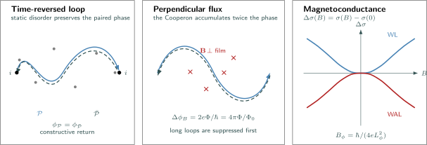
The weak-localization ledger. At zero field, a loop and its time reverse have equal phase and enhance return. Perpendicular flux creates a relative phase $4\pi\Phi/\Phi_0$ and suppresses the Cooperon. In the stated convention $\Delta\sigma(B)=\sigma(B)-\sigma(0)$, weak localization bends upward and weak antilocalization bends downward.

Quantum Correction to Conductivity

Return probability

The diffusion kernel in $d$ dimensions is

$$P(\mathbf r,t) = \frac{1}{(4\pi Dt)^{d/2}} \exp\!\left( -\frac{r^2}{4Dt} \right).$$

The return probability density is

$$P(\mathbf 0,t) = \frac{1}{(4\pi Dt)^{d/2}}.$$

Interference accumulates after motion becomes diffusive, $t\gtrsim\tau_{\mathrm{tr}}$, and is cut off after phase memory is lost, $t\gtrsim\tau_\phi$. The correction therefore has the structural form

$$\delta\sigma \propto -e^2D \int_{\tau_{\mathrm{tr}}}^{\tau_\phi} dt\, P(\mathbf0,t).$$

In two dimensions, $P(\mathbf0,t)\propto1/t$, so every logarithmic interval of return time contributes comparably:

$$\delta\sigma_{2\mathrm D} \propto -\ln \left( \frac{\tau_\phi}{\tau_{\mathrm{tr}}} \right).$$

This time-of-flight interpretation explains why low-temperature magnetotransport is sensitive to picosecond-to-nanosecond coherence even though each elastic collision occurs much earlier.

Cooperon mode integral

After disorder averaging, the path–reverse-path interference is represented by the Cooperon. In the simplest scalar channel,

$$C(\mathbf q,\omega) = \frac{1}{ Dq^2-i\omega+\tau_\phi^{-1} }.$$

The zero-frequency conductivity correction is

$$\delta\sigma = - \frac{2e^2D}{\pi\hbar} \int \frac{d^dq}{(2\pi)^d} \frac{1}{ Dq^2+\tau_\phi^{-1} },$$

where order-one channel and cutoff conventions must be stated. The ultraviolet cutoff is $q_{\max}\sim\ell_{\mathrm{tr}}^{-1}$. The infrared cutoff is set by

$$q_{\min} \sim \max \left( L_\phi^{-1}, L^{-1}, L_B^{-1}, L_s^{-1}, \ldots \right).$$

For a large two-dimensional sample in the elementary orthogonal case,

$$\delta\sigma_{2\mathrm D}(0) \simeq - \frac{e^2}{2\pi^2\hbar} \ln \left( \frac{\tau_\phi}{\tau_{\mathrm{tr}}} \right)$$

up to finite constants absorbed into the short-scale conductivity. Equivalently,

$$\delta\sigma_{2\mathrm D}(0) \simeq - \frac{e^2}{\pi^2\hbar} \ln \left( \frac{L_\phi}{\ell_{\mathrm{tr}}} \right)$$

when the length and time cutoffs are matched at logarithmic accuracy.

The correction must remain perturbative:

$$\left| \delta\sigma \right| \ll \sigma_{\mathrm D}.$$

Once it becomes comparable with the Drude value, a first-order weak-localization formula is not self-consistent.

Dimensional dependence

The same return integral behaves differently with dimension:

Effective dimension	Long-time return integral	Leading coherence dependence
quasi-1D	$\int dt\,t^{-1/2}$	$\delta G\propto-L_\phi/L$ after geometry factors
2D	$\int dt\,t^{-1}$	$\delta\sigma\propto-\ln(L_\phi/\ell)$
3D	$\int dt\,t^{-3/2}$	ultraviolet-dominated constant plus a term proportional to $+1/L_\phi$

The effective dimension is set by the diffusion length over the relevant time. A film is two-dimensional for the interference correction when

$$t_{\mathrm{film}} \ll L_\phi$$

and the magnetic and thermal lengths do not resolve its thickness. A narrow wire becomes quasi-one-dimensional when both transverse dimensions are smaller than the active coherence scale.

Magnetic-Field Suppression

The Cooperon sees charge twice

For a closed path enclosing flux

$$\Phi = \oint_{\mathcal P} \mathbf A\cdot d\mathbf l,$$

the orbital phase changes sign when the path is reversed. The relative phase is

$$\Delta\phi_B = \frac{2e}{\hbar}\Phi = 4\pi \frac{\Phi}{\Phi_0}, \qquad \Phi_0=\frac{h}{e}.$$

The factor $2e$ is not a Cooper-pair charge. It arises because the interference compares one electron path with its reverse. In the Cooperon equation, the gradient is correspondingly replaced by

$$-i\nabla \longrightarrow -i\nabla - \frac{2e}{\hbar}\mathbf A.$$

A perpendicular field quantizes the diffusive transverse modes:

$$Dq^2 \longrightarrow \frac{4eD\lvert B\rvert}{\hbar} \left( n+\frac12 \right).$$

The field scale associated with a decay time $\tau_i$ is

$$B_i = \frac{\hbar}{4eD\tau_i} = \frac{\hbar}{4eL_i^2}, \qquad L_i=\sqrt{D\tau_i}.$$

In particular,

$$B_\phi = \frac{\hbar}{4eD\tau_\phi} = \frac{\hbar}{4eL_\phi^2}.$$

Long coherent loops enclose larger areas and are destroyed by smaller fields.

Two-dimensional line shape

Define

$$\mathcal F(z) = \psi \left( \frac12+\frac{1}{z} \right) + \ln z, \qquad z>0,$$

where $\psi$ is the digamma function and $\mathcal F(0)$ is defined by continuity. A common single-scale convention is

$$\Delta\sigma(B) = \alpha \frac{e^2}{2\pi^2\hbar} \mathcal F \left( \frac{\lvert B\rvert}{B_\phi} \right).$$

At small field,

$$\mathcal F(z) = \frac{z^2}{24} - \frac{7z^4}{960} + O(z^6),$$

so the ideal orbital curve is even and quadratic at the origin. In the present sign convention:

$$\begin{array}{lll} \alpha>0 &\Rightarrow& \text{weak localization},\\[3pt] \alpha<0 &\Rightarrow& \text{weak antilocalization}. \end{array}$$

Other papers define $\Delta\sigma$ with the opposite order or place a minus sign in front of $\alpha$. Always read the equation before interpreting the fitted sign.

Worked field scale

Let

$$D = 0.020\ \mathrm{m^2\,s^{-1}}, \qquad \tau_\phi = 50\ \mathrm{ps}.$$

Then

$$L_\phi = \sqrt{D\tau_\phi} = 1.00\ \mu\mathrm m$$

and

$$B_\phi = \frac{\hbar}{4eL_\phi^2} \simeq 1.65\times10^{-4}\ \mathrm T = 0.165\ \mathrm{mT}.$$

A cusp much broader than this estimate requires a shorter coherent length, additional channel gaps, a different diffusion constant, or a fitting model outside the assumed geometry.

Weak Antilocalization

For spin-$1/2$ particles, time reversal satisfies

$$\mathcal T^2=-1.$$

Spin–orbit coupling rotates spin as momentum changes. The reversed trajectory retraces the orbital path but also carries a constrained spin rotation. In the symplectic regime, the net path–reverse-path interference can reduce return probability rather than enhance it. The conductivity correction is then positive at zero field, and suppressing it with field gives negative $\Delta\sigma(B)$ in the convention used here.

This is weak antilocalization. It remains a small interference correction:

$$\left| \delta\sigma_{\mathrm{WAL}} \right| \ll \sigma_{\mathrm D}.$$

The name does not mean that all states are extended, nor that strong disorder cannot eventually localize the system. It identifies the sign of the perturbative quantum correction in a symmetry regime.

A $\pi$ Berry phase can provide an equivalent language in some Dirac systems, but a WAL cusp is not unique evidence for a topological surface state. Rashba-split semiconductor bands, ordinary heavy-element films, coupled quantum wells, graphene valley structure, and several bulk channels can all produce WAL-like magnetoconductance.

Spin–Orbit and Internal Channels

Singlet and triplet Cooperons

The product of two spin-$1/2$ amplitudes decomposes into one singlet and three triplet Cooperon modes:

$$\frac12\otimes\frac12 = 0\oplus1.$$

Without spin relaxation, the channel sum produces the ordinary orthogonal correction. Spin–orbit coupling relaxes or mixes the triplet modes while the singlet has the opposite interference sign. In the strong spin–orbit limit, the surviving low-energy balance is antilocalizing.

A useful schematic channel formula is

$$\Delta\sigma(B) = \frac{e^2}{2\pi^2\hbar} \sum_a \alpha_a \mathcal F \left[ \frac{\lvert B\rvert}{ B_\phi+B_a } \right],$$

where

$$B_a = \frac{\hbar\Gamma_a}{4eD}$$

encodes a channel relaxation rate $\Gamma_a$. The coefficients $\alpha_a$ and the combinations entering $B_a$ must come from the microscopic symmetry problem. Replacing them by several unconstrained copies of one curve can fit noise while obscuring the physics.

In the simplified strong-spin–orbit two-dimensional convention, one independent coherent symplectic channel often contributes approximately

$$\alpha \simeq -\frac12.$$

This is a benchmark, not a universal channel counter. Interchannel scattering, unequal diffusion constants, magnetic scattering, finite thickness, Zeeman mixing, and partial coherence shift the fitted value.

Spin-relaxation mechanisms

For Elliott–Yafet relaxation, each momentum-scattering event has a small spin-mixing probability $b^2$, giving schematically

$$\frac{1}{\tau_{\mathrm{so}}} \sim \frac{b^2}{\tau_{\mathrm{tr}}}.$$

More frequent momentum scattering then causes faster spin relaxation.

For Dyakonov–Perel relaxation, carriers precess in a momentum-dependent spin–orbit field $\boldsymbol\Omega(\mathbf k)$ between collisions. In the motional-narrowing regime,

$$\frac{1}{\tau_{\mathrm{so}}} \sim \left\langle \Omega^2 \right\rangle \tau_{\mathrm{tr}}.$$

More frequent momentum scattering interrupts precession and can lengthen the spin lifetime. Gate-dependent Rashba coupling, Dresselhaus anisotropy, cubic terms, and several occupied subbands can require an Iordanskii–Lyanda-Geller–Pikus or related model rather than a scalar Hikami–Larkin–Nagaoka fit.

Valley, surface, and band structure

Internal degrees of freedom create additional interference channels:

• intervalley scattering in graphene can restore ordinary weak localization by coupling valleys;
• intravalley chirality and trigonal warping gap different graphene Cooperons;
• top and bottom surfaces of a thin topological insulator can behave as two channels only if their coherent coupling is weak;
• bulk and surface carriers with different $D$ and $\tau_\phi$ cannot generally be represented by one common $B_\phi$;
• magnetic order or magnetic impurities break time reversal and can suppress both WL and WAL.

The fitted $\alpha$ is therefore a compressed summary of a model, not a direct measurement of “the number of topological channels.”

From Measured Resistance to Conductivity

The measured sheet-resistance tensor must be inverted before fitting a conductivity formula:

$$\boldsymbol\sigma = \boldsymbol\rho^{-1}.$$

For an isotropic two-dimensional Hall bar,

$$\sigma_{xx} = \frac{\rho_{xx}}{ \rho_{xx}^2+\rho_{xy}^2 }, \qquad \sigma_{xy} = -\frac{\rho_{xy}}{ \rho_{xx}^2+\rho_{xy}^2 }.$$

Using $\Delta R_{xx}$ as if it were $\Delta\sigma_{xx}$ is justified only when Hall mixing and relative corrections are demonstrably negligible.

Before inversion, remove contact mixing by field symmetrization:

$$\rho_{xx}^{\mathrm{sym}}(B) = \frac{ \rho_{xx}^{\mathrm{raw}}(B) + \rho_{xx}^{\mathrm{raw}}(-B) }{2},$$

and antisymmetrize the Hall trace:

$$\rho_{xy}^{\mathrm{asym}}(B) = \frac{ \rho_{xy}^{\mathrm{raw}}(B) - \rho_{xy}^{\mathrm{raw}}(-B) }{2}.$$

A fitted field offset should be reported and physically bounded; silently recentering each trace can absorb hysteresis, trapped flux, or magnetic texture.

Experimental Analysis Workflow

1. Establish diffusion. Determine density, mobility, $\tau_{\mathrm{tr}}$, $\ell_{\mathrm{tr}}$, and $D$. Verify $\ell_{\mathrm{tr}}\ll L_\phi$ and $\lvert B\rvert\ll B_{\mathrm{tr}}$ in the fit window.
2. Determine effective dimension. Compare thickness and width with $L_\phi$, thermal length, and magnetic length at every temperature.
3. Prepare the tensor. Symmetrize and antisymmetrize raw data, propagate geometric uncertainty, and invert $\boldsymbol\rho$.
4. Fit the narrowest justified model. Start with a physically motivated channel structure and a field window that excludes classical background, oscillations, hysteresis, and superconducting fluctuations.
5. Test window stability. Vary the maximum field and point weighting. A parameter that drifts beyond uncertainty is model-dependent.
6. Inspect covariance. $B_\phi$, $B_{\mathrm{so}}$, channel prefactors, and polynomial backgrounds can be strongly correlated.
7. Vary temperature and gate voltage. Check whether $D$, carrier density, occupied subbands, and dimensionality change alongside the cusp.
8. Use field orientation. A two-dimensional orbital correction depends mainly on perpendicular field; parallel-field response can expose finite thickness, Zeeman effects, or magnetic scattering.
9. Separate interaction corrections. Electron–electron interactions also change conductivity and magnetoresistance. Fit them with their own temperature, Zeeman, and screening structure.
10. Cross-check coherence. Compare $L_\phi$ with fluctuation correlation fields, ring harmonics, or independent noise and thermometry measurements.

Evidence ladder

Claim	Minimum evidence
A low-field quantum-interference cusp exists	Reproducible, even-in-field conductivity feature above noise and contact-mixing controls
The cusp is diffusive WL or WAL	Valid scale hierarchy, correct dimensionality, stable fit window, and classical-background audit
Spin–orbit coupling controls the sign	Symmetry-resolved channel model plus gate, material, orientation, or independent spin evidence
The prefactor counts channels	Demonstrated weak interchannel coupling and comparable channel diffusion/coherence scales
The channel is topological	Independent band, surface, thickness, gating, and symmetry evidence; WAL alone is insufficient
$L_\phi(T)$ reveals a dephasing mechanism	Electron thermometry, stable geometry, broad temperature range, and cross-probe consistency

Common Mistakes

Mistake	Why it fails	Better practice
Calling the cusp Anderson localization	WL and WAL are perturbative metallic corrections	Check $g\gg1$ and link strong localization separately
Reading a resistance sign as a conductivity sign	Tensor inversion reverses the small-correction sign	Fit $\sigma_{xx}(B)$ under a declared convention
Treating $\alpha$ as an integer channel count	Coupled modes and unequal scales renormalize it	Model channel coupling and report covariance
Fitting beyond the diffusive field range	Electronic cyclotron dynamics replace Cooperon diffusion	Restrict $\lvert B\rvert/B_{\mathrm{tr}}$ and test stability
Ignoring the Hall component	$\rho_{xy}$ enters the tensor inverse	Measure and invert both tensor components
Fitting a polynomial background and cusp simultaneously without controls	Background curvature can trade against $B_\phi$	Constrain background using wider-field and temperature data
Calling WAL proof of topology	Ordinary spin–orbit-coupled bands also give WAL	Require independent topological evidence
Using bath temperature as electron temperature	Joule heating changes $\tau_\phi$	Measure current dependence and use in situ thermometry
Applying a 2D formula through a dimensional crossover	The mode integral changes functional form	Compare all transverse dimensions with active lengths
Ignoring magnetic impurities or order	Time-reversal breaking gaps Cooperons	Measure hysteresis, moments, orientation, and field history
Adding several identical HLN terms freely	The fit becomes nonidentifiable	Derive channel rates and share constrained parameters
Equating $\tau_{\mathrm{so}}$ with a qubit $T_2$	Cooperon spin relaxation is a transport-channel scale	State the observable and microscopic relaxation model

Exercises

1. Two-dimensional logarithm

Evaluate

$$I_{2\mathrm D} = \int_{1/L_\phi}^{1/\ell} \frac{d^2q}{(2\pi)^2} \frac{1}{Dq^2}.$$

Use it to recover the logarithmic weak-localization correction.

Solution

In polar coordinates,

$$\begin{aligned} I_{2\mathrm D} &= \frac{1}{(2\pi)^2} \int_0^{2\pi}d\theta \int_{1/L_\phi}^{1/\ell} \frac{q\,dq}{Dq^2}\\ &= \frac{1}{2\pi D} \ln \left( \frac{L_\phi}{\ell} \right). \end{aligned}$$

Substituting into the scalar Cooperon correction gives

$$\delta\sigma = - \frac{2e^2D}{\pi\hbar} I_{2\mathrm D} = - \frac{e^2}{\pi^2\hbar} \ln \left( \frac{L_\phi}{\ell} \right).$$

Since $L_\phi^2=D\tau_\phi$ and $\ell^2$ is proportional to $D\tau_{\mathrm{tr}}$ up to a dimensional factor,

$$\delta\sigma \simeq - \frac{e^2}{2\pi^2\hbar} \ln \left( \frac{\tau_\phi}{\tau_{\mathrm{tr}}} \right)$$

at logarithmic accuracy.

2. Magnetic phase of a reversed loop

Show that the orbital phase difference between a closed electron path and its reverse is $2e\Phi/\hbar$. What flux gives a phase difference of order one?

Solution

For electron charge $-e$, the vector-potential phase is

$$\phi_{\mathcal P}^{(B)} = -\frac{e}{\hbar} \oint_{\mathcal P} \mathbf A\cdot d\mathbf l = -\frac{e\Phi}{\hbar}.$$

Reversing the path reverses the line integral:

$$\phi_{\bar{\mathcal P}}^{(B)} = +\frac{e\Phi}{\hbar}.$$

Their difference has magnitude

$$\lvert\Delta\phi_B\rvert = \frac{2e\lvert\Phi\rvert}{\hbar} = 4\pi \frac{\lvert\Phi\rvert}{\Phi_0}.$$

Suppression begins when this is of order one, so the relevant flux is of order

$$\lvert\Phi\rvert \sim \frac{\hbar}{2e} = \frac{\Phi_0}{4\pi}.$$

Exact line-shape factors come from averaging the distribution of loop areas, not from setting one sharp flux threshold.

3. Coherence field

A film has $D=0.010\ \mathrm{m^2\,s^{-1}}$ and $\tau_\phi=20\ \mathrm{ps}$. Find $L_\phi$ and $B_\phi$.

Solution

The coherence length is

$$L_\phi = \sqrt{D\tau_\phi} = \sqrt{ (0.010)(20\times10^{-12}) } \simeq 4.47\times10^{-7}\ \mathrm m.$$

Thus

$$L_\phi \simeq 447\ \mathrm{nm}.$$

The field is

$$\begin{aligned} B_\phi &= \frac{\hbar}{4eL_\phi^2}\\ &\simeq \frac{ 1.055\times10^{-34} }{ 4(1.602\times10^{-19})(2.00\times10^{-13}) }\\ &\simeq 8.23\times10^{-4}\ \mathrm T. \end{aligned}$$

Therefore

$$B_\phi \simeq 0.823\ \mathrm{mT}.$$

4. Small-field curvature

Use the large-argument expansion of the digamma function to show

$$\mathcal F(z) = \frac{z^2}{24} + O(z^4).$$

What is $\Delta\sigma/(e^2/h)$ at $\lvert B\rvert=0.2B_\phi$ for $\alpha=1$ at leading order?

Solution

For $x\gg1$,

$$\psi \left( x+\frac12 \right) = \ln x + \frac{1}{24x^2} + O(x^{-4}).$$

Set $x=1/z$. Then

$$\mathcal F(z) = \psi \left( \frac12+\frac1z \right) + \ln z = \frac{z^2}{24} + O(z^4).$$

At $z=0.2$,

$$\mathcal F(0.2) \simeq \frac{0.2^2}{24} = 1.667\times10^{-3}.$$

Because

$$\frac{ e^2/(2\pi^2\hbar) }{ e^2/h } = \frac1\pi,$$

the leading correction is

$$\frac{\Delta\sigma}{e^2/h} \simeq \frac{\mathcal F(0.2)}{\pi} \simeq 5.31\times10^{-4}.$$

5. Conductivity and resistance signs

A weak-localization film has $\Delta\sigma_{xx}(B)>0$ and negligible Hall response. Show the sign of $\Delta\rho_{xx}(B)$ to first order.

Solution

Write

$$\sigma(B) = \sigma_0+\Delta\sigma(B), \qquad \lvert\Delta\sigma\rvert\ll\sigma_0.$$

Then

$$\begin{aligned} \rho(B) &= \frac{1}{\sigma_0+\Delta\sigma}\\ &\simeq \frac1{\sigma_0} - \frac{\Delta\sigma}{\sigma_0^2}. \end{aligned}$$

Therefore

$$\Delta\rho(B) \simeq -\rho_0^2\Delta\sigma(B) < 0.$$

Weak localization gives positive magnetoconductance and negative magnetoresistance in this limit.

6. Dimensional crossover

A film is $30\ \mathrm{nm}$ thick. Its fitted $L_\phi$ decreases from $600\ \mathrm{nm}$ at $1\ \mathrm K$ to $20\ \mathrm{nm}$ at $40\ \mathrm K$. Can one use one two-dimensional formula throughout?

Solution

At $1\ \mathrm K$,

$$t_{\mathrm{film}} \ll L_\phi,$$

so coherent diffusion does not resolve the thickness and a two-dimensional orbital treatment can be appropriate.

At $40\ \mathrm K$,

$$L_\phi < t_{\mathrm{film}},$$

so the coherent paths explore the thickness. The mode spectrum crosses toward three dimensions, and a two-dimensional digamma fit is no longer justified without a finite-thickness calculation. The crossover may occur before $L_\phi=t_{\mathrm{film}}$ if the magnetic or thermal length becomes the shorter resolving scale.

7. Coupled WAL channels

Two equivalent, independent symplectic surfaces each have $\alpha=-1/2$. What prefactor is expected if they are independent? What can happen when coherent intersurface scattering is much faster than dephasing?

Solution

Independent corrections add:

$$\alpha_{\mathrm{tot}} = -\frac12-\frac12 = -1.$$

If coherent intersurface scattering is fast, the two surface labels are not separately conserved over $\tau_\phi$. One symmetric long-lived Cooperon combination can remain while the orthogonal combination is gapped. The low-field response can then approach

$$\alpha_{\mathrm{tot}} \simeq -\frac12.$$

Intermediate coupling, unequal $D$, bulk mediation, or magnetic scattering gives nonuniversal values. Thus observing $\alpha=-1$ or $-1/2$ does not by itself prove two or one topological surfaces.

8. Audit a WAL fit

A paper fits a sharp resistance cusp from $-2$ to $2\ \mathrm T$ with a single two-dimensional HLN curve and reports $\alpha=-3.7$ and $L_\phi=4\ \mu\mathrm m$. No Hall data, diffusion constant, sample thickness, fit-window test, or electron-temperature check is shown. Identify at least eight problems.

Solution

The analysis should be challenged because:

1. a conductivity formula was applied directly to resistance;
2. the Hall tensor was not measured or inverted;
3. $D$ and $\tau_{\mathrm{tr}}$ are absent, so $B_{\mathrm{tr}}$ and diffusive validity are unknown;
4. a $2\ \mathrm T$ window may be far outside the low-field Cooperon regime;
5. thickness was not compared with $L_\phi$ or magnetic length;
6. $\alpha=-3.7$ was not tied to a microscopic channel model;
7. classical multiband magnetoresistance and background curvature were not separated;
8. fit-window stability and parameter covariance were not reported;
9. the inferred $L_\phi$ lacks a consistency check against device size;
10. electron overheating and current dependence were not tested;
11. magnetic hysteresis or field offset was not audited;
12. interaction, superconducting-fluctuation, and conductance-fluctuation corrections were not excluded.

A numerically good curve is not enough when its scale hierarchy and observable conversion are unspecified.

Connections

• Anderson Localization owns the nonperturbative regime of exponentially localized states and typical conductance.
• Scaling Theory of Localization promotes the perturbative logarithm to a scale flow and develops its dimensional, fixed-point, and critical consequences.
• Disorder in Quantum Matter defines the elastic, quantum, transport, and magnetic disorder scales entering the Cooperon.
• Quantum Coherence in Conductors develops dephasing mechanisms, thermal averaging, dimensionality, and cross-probe coherence tests.
• Universal Conductance Fluctuations treats sample-specific interference around the same diffusive saddle.
• Aharonov–Bohm Rings resolves fixed-winding paths and $h/e$ or $h/2e$ harmonics rather than the broad loop-area ensemble.
• Drude Theory supplies the classical conductivity baseline and tensor inversion conventions.
• Transport Measurements supplies current and field reversal, geometry conversion, reciprocity, sweep-rate, heating, and uncertainty checks for the magnetotransport record.
• Kubo Formula owns the exact linear-response framework from which disorder diagrams and vertex corrections are organized.
• Graphene and Dirac Materials supplies valley, chirality, Berry phase, intervalley scattering, and Dirac-band context.
• Graphene classifies the strain, substrate, mass, and intervalley operators that determine which graphene interference channels survive in a device.
• Spin–Orbit Coupling develops the microscopic coupling of spin to orbital motion before its diffusive transport reduction.

References

1. L. P. Gor’kov, A. I. Larkin, and D. E. Khmel’nitskii, “Particle Conductivity in a Two-Dimensional Random Potential,” JETP Letters 30, 228–232 (1979). Establishes the singular interference correction in two-dimensional disorder.
2. E. Abrahams, P. W. Anderson, D. C. Licciardello, and T. V. Ramakrishnan, “Scaling Theory of Localization: Absence of Quantum Diffusion in Two Dimensions,” Physical Review Letters 42, 673–676 (1979), doi:10.1103/PhysRevLett.42.673. Connects the perturbative correction to conductance scaling.
3. S. Hikami, A. I. Larkin, and Y. Nagaoka, “Spin–Orbit Interaction and Magnetoresistance in the Two Dimensional Random System,” Progress of Theoretical Physics 63, 707–710 (1980), doi:10.1143/PTP.63.707. Derives the canonical two-dimensional field and spin–orbit structure.
4. A. Kawabata, “Theory of Negative Magnetoresistance in Three-Dimensional Systems,” Solid State Communications 34, 431–432 (1980), doi:10.1016/0038-1098(80)90644-4. Extends field suppression to three dimensions.
5. B. L. Altshuler, A. G. Aronov, and D. E. Khmelnitsky, “Effects of Electron–Electron Collisions with Small Energy Transfers on Quantum Localisation,” Journal of Physics C: Solid State Physics 15, 7367–7386 (1982), doi:10.1088/0022-3719/15/36/018. Develops interaction-induced phase relaxation.
6. G. Bergmann, “Weak Localization in Thin Films: A Time-of-Flight Experiment with Conduction Electrons,” Physics Reports 107, 1–58 (1984), doi:10.1016/0370-1573(84)90103-0. Classic physical and experimental review.
7. P. A. Lee and T. V. Ramakrishnan, “Disordered Electronic Systems,” Reviews of Modern Physics 57, 287–337 (1985), doi:10.1103/RevModPhys.57.287. Reviews localization, interactions, and transport corrections.
8. C. W. J. Beenakker and H. van Houten, “Quantum Transport in Semiconductor Nanostructures,” Solid State Physics 44, 1–228 (1991), doi:10.1016/S0081-1947(08)60091-0. Provides mesoscopic transport, coherence, and geometry context.
9. S. V. Iordanskii, Yu. B. Lyanda-Geller, and G. E. Pikus, “Weak Localization in Quantum Wells with Spin–Orbit Interaction,” JETP Letters 60, 206–210 (1994). Develops spin-precession channel structure beyond a scalar spin-flip time.
10. W. Knap, C. Skierbiszewski, A. Zduniak, et al., “Weak Antilocalization and Spin Precession in Quantum Wells,” Physical Review B 53, 3912–3924 (1996), doi:10.1103/PhysRevB.53.3912. Tests spin–orbit interference in semiconductor wells.
11. E. McCann, K. Kechedzhi, V. I. Fal’ko, H. Suzuura, T. Ando, and B. L. Altshuler, “Weak-Localization Magnetoresistance and Valley Symmetry in Graphene,” Physical Review Letters 97, 146805 (2006), doi:10.1103/PhysRevLett.97.146805. Resolves graphene valley and chirality channels.
12. F. V. Tikhonenko, D. W. Horsell, R. V. Gorbachev, and A. K. Savchenko, “Weak Localization in Graphene Flakes,” Physical Review Letters 100, 056802 (2008), doi:10.1103/PhysRevLett.100.056802. Experimental channel and dephasing analysis in graphene.
13. S. Pierre, A. B. Gougam, A. Anthore, H. Pothier, D. Esteve, and N. O. Birge, “Dephasing of Electrons in Mesoscopic Metal Wires,” Physical Review B 68, 085413 (2003), doi:10.1103/PhysRevB.68.085413. Demonstrates careful low-temperature coherence extraction and saturation controls.
14. J. Wang, X. Liu, C. Bunker, et al., “Weak Antilocalization Beyond the Fully Diffusive Regime in Topological Quantum Wells,” Physical Review B 102, 155307 (2020), doi:10.1103/PhysRevB.102.155307. Shows explicitly where the standard diffusive HLN model ceases to apply.
15. J. Liao, Y. Ou, X. Feng, et al., “Observation of Anderson Localization in Ultrathin Films of Three-Dimensional Topological Insulators,” Physical Review Letters 114, 216601 (2015), doi:10.1103/PhysRevLett.114.216601. Tracks a disorder-driven crossover from WAL to hopping transport.

Further Reading

• E. Akkermans and G. Montambaux, Mesoscopic Physics of Electrons and Photons, Cambridge University Press, 2007. A systematic path, Diffuson, Cooperon, and field-theory treatment.
• Y. Imry, Introduction to Mesoscopic Physics, 2nd ed., Oxford University Press, 2002. A compact physical account of coherence and disordered conductance.
• S. Datta, Electronic Transport in Mesoscopic Systems, Cambridge University Press, 1995. Connects scattering matrices, reservoirs, and coherent device transport.