Transport Measurements

An electrical transport measurement drives charge through a material and records terminal voltages or currents as functions of temperature, magnetic field, angle, frequency, gate voltage, pressure, and excitation amplitude. Its most immediate observable is a terminal response, not a scattering time, carrier density, mobility, gap, or phase. Those material inferences require a geometry model, a transport regime, a calibrated protocol, and checks that the sample remained in linear response and near the intended thermodynamic state.

For current sent into terminal $i$ and removed from terminal $j$, define $I_{ij}>0$. If the voltage leads read $V_k-V_l$, the measured transfer resistance is

$$R_{ij,kl} = \left. \frac{V_k-V_l}{I_{ij}} \right|_{\mathcal P},$$

where $\mathcal P$ denotes the complete protocol: wiring, temperature, magnetic field, field history, excitation frequency, current amplitude, delay, filtering, and averaging. Writing the terminal indices prevents a common category error: two contact configurations on the same sample need not measure the same resistance.

Canonical Scope

This page is the canonical home for low-frequency electrical transport practice in quantum matter: two- and four-terminal geometries, longitudinal resistance, conversion to sheet resistance or bulk resistivity, contact and loading effects, dc reversal and lock-in methods, temperature and field sweeps, uncertainty budgets, and common failure modes.

How Quantum Matter Is Measured owns the probe-independent measurement contract. The Transport, Response, and Optics gateway selects among bulk, kinetic, correlation, and coherent-terminal descriptions. Drude Theory and Boltzmann Transport own relaxation-time and kinetic descriptions; Kubo Formula owns exact linear response. Hall Effect owns ordinary and anomalous Hall physics, while Hall Measurements owns detailed transverse-voltage reduction. Quantum Oscillations owns inverse-field transforms, Lifshitz–Kosevich fits, orbit reconstruction, and phase analysis. Conductance Quantization owns coherent Landauer channels, for which a local bulk resistivity can cease to be the useful description.

The Measurement Contract

A reproducible transport dataset should identify at least:

• sample: composition, dimensions, thickness convention, crystal axes, contact layout, substrate, gate stack, and thermal cycle;
• source: current- or voltage-bias mode, waveform, amplitude, frequency, compliance, source impedance, and reversal sequence;
• detector: voltage or current range, input impedance, bandwidth, filtering, phase convention, and calibration;
• environment: sample temperature, thermometer location, magnetic-field vector, pressure, illumination, and sweep history;
• reduction: offset subtraction, symmetrization, geometry conversion, tensor inversion, interpolation, and rejected points;
• uncertainty: repeatability, drift, calibration, geometry, alignment, temperature, field, and model dependence.

A plot labeled only “resistivity versus temperature” omits most of this contract. The missing information may determine whether another laboratory can reproduce either the curve or its interpretation.

Four-Terminal Geometry

Two terminals mix several voltage drops

In a two-terminal measurement, the same pair of wires carries the source current and senses the voltage. In a simple lumped model,

$$\begin{aligned} V_{\mathrm{2t}} ={}& V_{\mathrm{off}} + I\bigl( R_{\mathrm{s}} +R_{\mathrm{c1}}+R_{\mathrm{c2}} \\ &\qquad\quad +R_{\mathrm{l1}}+R_{\mathrm{l2}} \bigr), \end{aligned}$$

where $R_{\mathrm{s}}$ is the intended sample contribution, $R_{\mathrm{c}}$ denotes contact or spreading resistance, $R_{\mathrm{l}}$ denotes lead resistance, and $V_{\mathrm{off}}$ collects thermoelectric and instrumental offsets. Two-terminal resistance is often the correct device observable, but it is generally not a bulk resistivity.

Separate current and voltage leads

In a four-terminal measurement, one pair of contacts sources $I_{ij}$ and another pair senses $V_k-V_l$. A voltmeter with input impedance $Z_{\mathrm{in}}$ draws only a small sense current. Consequently, voltage-lead and voltage-contact drops are suppressed by the ratio of their resistance to $Z_{\mathrm{in}}$.

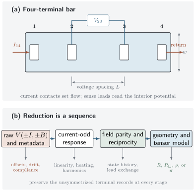
Four-terminal transport separates current injection from voltage sensing. The lower panel emphasizes that current reversal, field parity, and geometry conversion are distinct operations. Four terminals reject series lead drops only under the high-input-impedance approximation; they do not make contacts, current distribution, or sample geometry irrelevant.

Four-terminal sensing does not guarantee a noninvasive measurement. Current contacts can still:

• inject through a barrier or a nonlinear interface;
• create current crowding near a narrow contact;
• heat the electron system or the lattice;
• short part of a thin flake or edge channel;
• dope, strain, chemically modify, or electrostatically screen the sample;
• force current through an inhomogeneous percolation path.

Voltage contacts can also perturb a mesoscopic conductor even when their dc input current is small. In a coherent device, a voltage probe is a boundary condition and reservoir, not merely an ideal observer. Multi-terminal conductance must then be analyzed with the Landauer–Büttiker framework.

Longitudinal Resistance

Resistance is configuration dependent

“Longitudinal” means that the voltage separation is intended to follow the mean current direction. The adjective does not prove that the measured voltage contains only a longitudinal electric field. Misaligned contacts, anisotropy, inhomogeneous current flow, and transverse response can all contribute.

For a nonlinear current–voltage curve, distinguish the chord and differential resistances:

$$R_{\mathrm{chord}}(I) = \frac{V(I)}{I}, \qquad r_{\mathrm{diff}}(I_0) = \left. \frac{dV}{dI} \right|_{I_0}.$$

They agree only in a linear regime after offsets have been handled. A lock-in amplifier measures a small-signal differential response around its operating point, not automatically the full ratio $V/I$.

Field parity is a diagnostic, not a universal correction

In a nonmagnetic sample in a reversible state, an intended longitudinal channel is commonly even in magnetic field, whereas an ordinary Hall admixture is odd. One therefore forms

$$\begin{aligned} R^{\mathrm{even}}(B) &= \frac{R(+B)+R(-B)}{2}, \\ R^{\mathrm{odd}}(B) &= \frac{R(+B)-R(-B)}{2}. \end{aligned}$$

This decomposition is algebraically exact, but naming the pieces “longitudinal” and “Hall” adds physical assumptions. It can fail when magnetization, domains, metastability, or the sample temperature differ between the two field points.

The stronger linear-response check is Onsager–Casimir reciprocity. With all time-reversal-odd internal variables represented collectively by $\mathcal M$,

$$R_{ij,kl}(B,\mathcal M) = R_{kl,ij}(-B,-\mathcal M).$$

Testing reciprocal lead configurations can reveal wiring errors, drift, nonlinearity, or a state that was not reversed. Reciprocity is not a license to average genuinely hysteretic branches into one curve.

From Resistance to Conductivity

Uniform rectangular bar

If current density is uniform along a homogeneous bar of width $w$, thickness $t$, and voltage-probe separation $L$, then

$$\rho_{xx} = R_{xx}\frac{wt}{L}, \qquad \sigma_{xx} = \rho_{xx}^{-1}$$

only when the scalar approximation is valid. The measured $R_{xx}$ has units of ohms; the three-dimensional resistivity $\rho_{xx}$ has units of $\Omega\,\mathrm m$.

This conversion assumes that:

• the current contacts establish nearly uniform flow before the voltage region;
• $w$ and $t$ describe the electrically active cross section;
• voltage contacts are small compared with $L$;
• the material is homogeneous over the sampled region;
• nonlocal and ballistic effects are negligible;
• off-diagonal tensor components do not alter the conversion.

Violation of these assumptions calls for a Laplace-equation, finite-element, conformal-mapping, or multi-terminal model rather than a more precise measurement of the same geometric dimensions.

Thin films and sheet resistance

For a uniform film,

$$R_{\square} \equiv \frac{\rho}{t}, \qquad R_{xx} = R_{\square}\frac{L}{w}.$$

$R_{\square}$ is called sheet resistance and is reported in ohms, often annotated as $\Omega/\square$ to remind the reader that a square has $L/w=1$. “Ohms per square” is not a new SI dimension. When conduction occupies several parallel layers or a thickness-dependent surface region, converting $R_{\square}$ to a bulk $\rho$ using the physical thickness can be misleading.

van der Pauw extraction

For a homogeneous, isotropic, simply connected sheet of uniform thickness with sufficiently small contacts on its boundary, two transfer resistances $R_A$ and $R_B$ determine $R_{\square}$ through

$$\exp\!\left( -\frac{\pi R_A}{R_{\square}} \right) + \exp\!\left( -\frac{\pi R_B}{R_{\square}} \right) = 1.$$

When $R_A=R_B=R_0$, this reduces to

$$R_{\square} = \frac{\pi R_0}{\ln 2}.$$

The formula does not excuse large interior contacts, holes, thickness gradients, anisotropy, or inhomogeneity. Reversal and reciprocal configurations provide valuable internal checks before the nonlinear equation is solved. Anisotropic rectangular samples may instead require a Montgomery analysis or a numerical current-flow model with the crystal axes and contact geometry stated explicitly.

Conductivity is a tensor inverse

In a magnetic field or anisotropic crystal,

$$\mathbf E = \boldsymbol{\rho}\,\mathbf J, \qquad \mathbf J = \boldsymbol{\sigma}\,\mathbf E, \qquad \boldsymbol{\sigma} = \boldsymbol{\rho}^{-1}.$$

Tensor inversion is not elementwise inversion. For an in-plane isotropic system with antisymmetric transverse response,

$$\begin{aligned} \sigma_{xx} &= \frac{\rho_{xx}} {\rho_{xx}^{\,2}+\rho_{xy}^{\,2}}, \\ \sigma_{xy} &= -\frac{\rho_{xy}} {\rho_{xx}^{\,2}+\rho_{xy}^{\,2}}. \end{aligned}$$

Replacing $\sigma_{xx}$ by $1/\rho_{xx}$ is justified only when $|\rho_{xy}|\ll|\rho_{xx}|$ or when symmetry removes the transverse component. Sign conventions for $\rho_{xy}$ and $\sigma_{xy}$ must be declared rather than inferred from a plot.

Excitation and Readout

Current reversal

At fixed environment, expand the measured voltage around zero current:

$$V(I) = V_0 +R_1 I +a_2 I^2 +a_3 I^3 +\cdots .$$

The current-odd and current-even combinations are

$$\begin{aligned} V_{\mathrm{odd}}(I) &= \frac{V(+I)-V(-I)}{2}, \\ V_{\mathrm{even}}(I) &= \frac{V(+I)+V(-I)}{2}. \end{aligned}$$

A static thermoelectric offset enters $V_{\mathrm{even}}$, so $V_{\mathrm{odd}}/I$ estimates $R_1$ at sufficiently small $I$. Current reversal does not remove odd nonlinearities such as $a_3I^3$, nor does it guarantee that the sample returns to the same temperature or state between polarities. Measuring several amplitudes is more informative than trusting one reversed pair.

Useful sequence checks include $+I,0,-I,0$ or interleaved positive and negative currents. Zero-current readings track drift, while randomized or symmetric ordering reduces bias from a monotonic temperature drift. Waiting times must exceed the relevant electrical and thermal settling times.

AC and lock-in measurements

With a sinusoidal current $I(t)=I_0\cos\omega t$, phase-sensitive detection extracts the voltage component at the reference frequency. Define the complex transfer impedance

$$Z_{ij,kl}(\omega) = \frac{\widetilde V_{kl}^{(1)}(\omega)} {\widetilde I_{ij}^{(1)}(\omega)}.$$

Its in-phase part approaches the dc transfer resistance only when the sample, wiring, filters, preamplifier, and lock-in are all in a quasistatic regime. Stray capacitance, inductive pickup, dielectric loss, and phase errors can produce a quadrature signal or frequency dependence unrelated to intrinsic material dynamics.

Lock-in detection narrows the effective noise bandwidth, but it does not know which signal at the reference frequency came from the sample. Capacitive pickup from the source line, ground loops, vibration in a field gradient, and temperature modulation can all be phase coherent. Tests at several frequencies, cable configurations, and time constants are therefore part of the measurement rather than optional instrumentation details.

Higher harmonics are diagnostics. A voltage at $3\omega$ can arise from cubic electrical response or from Joule heating combined with $dR/dT$; a response at $2\omega$ can reveal an even-in-current process, asymmetric contacts, or thermoelectric conversion. The harmonic label alone does not identify a mechanism.

Noise, bandwidth, and loading

For a resistor in equilibrium, the classical low-frequency Johnson–Nyquist voltage-noise estimate over bandwidth $\Delta f$ is

$$v_{\mathrm n,rms} = \sqrt{4k_{\mathrm B}TR\,\Delta f}.$$

Real measurements add amplifier voltage and current noise, source noise, contact fluctuations, environmental pickup, digitization, and low-frequency drift. Increasing current raises the signal linearly but the Joule power quadratically:

$$P_{\mathrm J} = IV \simeq I^2R.$$

The useful excitation lies between a noise floor and a perturbation ceiling. Demonstrating an amplitude-independent resistance over a stated range is stronger evidence for linear response than quoting the smallest available current.

Finite voltmeter input impedance causes loading, especially for highly resistive samples. Leakage through cables, filters, substrates, cryostat wiring, or gate dielectrics can then compete with the sample current. Guarding and insulation help, but an open-circuit and dummy-load test are needed to quantify the background path.

Temperature Sweeps

The thermometer reports its own temperature. The sample temperature agrees only after thermal gradients and time constants are controlled. A trustworthy temperature sweep records:

• thermometer identity, calibration, mounting, and distance from the sample;
• heating or cooling direction and sweep rate;
• stabilization criterion or dwell time;
• excitation amplitude and dissipated power;
• vacuum, exchange gas, or thermal-link conditions;
• repeated cycles and any irreversible sample change.

Near a sharp transition, a continuous sweep can turn thermal lag into an apparent hysteresis or shift. Compare warming and cooling at several rates, then repeat selected points after full stabilization. A current-dependence check separates an intrinsic transition width from self-heating or depinning.

Common summaries require care:

• Residual-resistivity ratio: a ratio such as $\rho(300\,\mathrm K)/\rho(T_{\mathrm{low}})$ can compare samples when the same geometry remains valid, but it does not uniquely measure one defect density or scattering mechanism.
• Activated behavior: a straight segment of $\ln R$ versus $1/T$ is evidence for an effective scale over that interval, not proof of a unique band gap. Contact freeze-out, parallel conduction, variable-range hopping, and temperature-dependent geometry are alternatives.
• Zero resistance: a value below the instrumental resolution supports a percolating low-resistance path. Bulk superconductivity requires complementary magnetic or thermodynamic evidence.
• Linear-in-temperature resistance: the fitted interval, intercept, current dependence, geometry, and competing power laws must be reported before attaching a microscopic “strange-metal” mechanism.

Magnetic-Field and Angle Sweeps

A field sweep changes more than the Hamiltonian. Moving flux induces voltage,

$$V_{\mathrm{ind}} = -\frac{d\Phi}{dt},$$

while eddy currents heat metallic structures and magnetocaloric effects can shift the sample temperature. Magnetic domains, vortices, and first-order transitions can retain field history. A complete protocol therefore records sweep direction, rate, maximum excursion, zero-field preparation, magnet polarity, persistent-switch state, and sample temperature during the sweep.

For longitudinal magnetotransport:

1. measure both field polarities with the same wiring;
2. repeat with current reversal or low-frequency phase-sensitive detection;
3. inspect even and odd field components without automatically discarding either;
4. exchange current and voltage terminals to test reciprocity where applicable;
5. vary sweep rate and excitation to test heating and dynamics;
6. repeat representative points after stabilized field steps.

An angle sweep needs a coordinate convention and a misalignment estimate. A small perpendicular component can dominate a nominally in-plane measurement in a high-mobility two-dimensional system. Mechanical backlash and sample rotation relative to thermometry or wiring can add apparent angular structure.

What a Typical Dataset Should Contain

A defensible transport dataset is usually a family of records, not one polished curve:

• current–voltage traces: establish the linear range, offsets, differential response, compliance events, and hysteresis;
• resistance versus temperature: includes both sweep directions, selected equilibrated points, and several excitation amplitudes;
• resistance versus field: includes both polarities and directions, raw and parity-decomposed channels, and the actual field history;
• frequency and phase scans: separate a quasistatic plateau from cable or filter response;
• configuration checks: compare lead permutations, contact pairs, reciprocal arrangements, and nominally equivalent devices;
• geometry records: microscopy or profilometry establishes $L$, $w$, $t$, contact size, cracks, and active regions;
• metadata: preserves source range, preamplifier gain, lock-in time constant, filter slope, sampling interval, thermometer, and calibration versions.

The raw voltage should remain available. Publishing only a geometry-normalized or background-subtracted trace makes it difficult to detect sign errors, clipping, offsets, or a mistaken thickness.

Interpretation Workflow

1. Inspect raw records. Check source compliance, detector overload, discontinuities, drift, and missing metadata before fitting.
2. Establish the response regime. Use several positive and negative currents; determine whether $V_{\mathrm{odd}}$ is proportional to $I$ and whether the inferred resistance is frequency independent.
3. Audit contacts and geometry. Compare configurations, reciprocal measurements, imaging, and dimensions. Decide whether a bar, van der Pauw, finite-element, or multi-terminal model is justified.
4. Separate symmetry channels. Apply current and field reversals as explicit algebraic operations. Preserve the unsymmetrized data and treat hysteretic states separately.
5. Convert quantities with units. State whether the result is resistance, conductance, sheet resistance, resistivity, or a tensor component. Propagate geometric uncertainty.
6. Identify the transport regime. Test whether a local diffusive constitutive law is appropriate. Ballistic, hydrodynamic, hopping, localized, edge-dominated, and superconducting transport require different inferences.
7. Compare competing models. Drude Theory, Boltzmann Transport, Weak Localization, and coherent channel theory predict different dependencies and validity ranges.
8. Seek orthogonal evidence. Transport is strongly weighted toward connected conducting paths. Spectroscopy, thermodynamics, microscopy, or scattering may be needed to establish a bulk gap, order parameter, carrier reconstruction, or phase volume.

Uncertainty Budget

For a uniform bar with $\rho=Rwt/L$, an independent-input approximation gives

$$\begin{aligned} \left( \frac{u_\rho}{\rho} \right)^2 \simeq{}& \left( \frac{u_R}{R} \right)^2 + \left( \frac{u_w}{w} \right)^2 \\ &+ \left( \frac{u_t}{t} \right)^2 + \left( \frac{u_L}{L} \right)^2. \end{aligned}$$

Correlated dimensions require covariance terms. More importantly, this expression covers parameter uncertainty within the bar model; it does not quantify bias from current crowding, parallel channels, cracks, an electrically inactive thickness, or a wrong constitutive regime.

A useful uncertainty ledger separates:

• repeatability: short-term scatter under an unchanged protocol;
• drift: changes with time, temperature, contact aging, or thermal cycling;
• instrument calibration: source current, voltage gain, phase, field, and thermometer;
• geometry: contact separation, width, thickness, edge roughness, and active cross section;
• state preparation: field history, sweep direction, dwell time, illumination, and gate history;
• model discrepancy: current distribution, tensor structure, parallel channels, and nonlocality.

Report enough significant figures to reflect this budget. A nanovoltmeter can resolve many digits while the sample thickness remains uncertain by ten percent.

Common Mistakes

• Calling every four-terminal ratio a resistivity without a geometry and regime model.
• Saying four-terminal sensing “removes contact resistance” without stating the high-input-impedance approximation or checking contact invasiveness.
• Using $1/\rho_{xx}$ for $\sigma_{xx}$ when transverse response is appreciable.
• Symmetrizing field data across branches that occupy different magnetic, vortex, or metastable states.
• Removing a voltage offset from one current polarity instead of measuring both polarities.
• Assuming current reversal removes self-heating and every nonlinear response.
• Choosing a lock-in frequency for convenience without checking phase and frequency dependence.
• Treating the thermometer reading as the sample temperature during a fast sweep.
• Converting sheet resistance to bulk resistivity with an unverified electrical thickness.
• Inferring bulk superconductivity, a carrier gap, or a microscopic scattering mechanism from transport alone.
• Subtracting an empirical background until the residual resembles a desired theory.
• Omitting raw terminal data, wiring indices, rejected sweeps, or negative results.

Exercises

1. Two-terminal and four-terminal resistance

A sample has $R_{\mathrm s}=12\,\mathrm{m}\Omega$. Each current contact contributes $0.35\,\Omega$, and each current lead contributes $0.08\,\Omega$. Ignore voltage offsets. What does the two-terminal measurement read? What ideal four-terminal value is obtained when the sense current is negligible?

Solution

The two-terminal path contains the sample, two contacts, and two leads:

$$\begin{aligned} R_{\mathrm{2t}} &= 0.012+2(0.35)+2(0.08) \\ &= 0.872\,\Omega. \end{aligned}$$

The ideal four-terminal voltage probes sample only the potential difference across the intended sample region, so

$$R_{\mathrm{4t}} = 12\,\mathrm{m}\Omega.$$

This answer assumes the current contacts do not alter the current distribution or heat the sample. Four terminals reject their series voltage drops; they do not prove that the contacts are physically noninvasive.

2. Current reversal

At $I=100\,\mu\mathrm A$, a voltmeter reads $V(+I)=1.545\,\mathrm{mV}$ and $V(-I)=-1.455\,\mathrm{mV}$. Find the current-odd voltage, the current-even voltage, and the linear-resistance estimate.

Solution

The odd and even combinations are

$$\begin{aligned} V_{\mathrm{odd}} &= \frac{1.545-(-1.455)}{2}\,\mathrm{mV} \\ &= 1.500\,\mathrm{mV}, \\ V_{\mathrm{even}} &= \frac{1.545+(-1.455)}{2}\,\mathrm{mV} \\ &= 0.045\,\mathrm{mV}. \end{aligned}$$

Therefore

$$R_1 \simeq \frac{V_{\mathrm{odd}}}{I} = 15.0\,\Omega.$$

The $45\,\mu\mathrm V$ even component is consistent with a static offset or an even-in-current effect. A second current amplitude is needed to test whether the odd response is truly linear.

3. Geometry and uncertainty

A bar gives $R=200\,\Omega$ with $L=1.00\,\mathrm{mm}$, $w=20.0\,\mu\mathrm m$, and $t=8.0\,\mathrm{nm}$. Find $\rho$. If the independent relative standard uncertainties in $R,w,t,L$ are $1\%,2\%,10\%,1\%$, estimate the relative uncertainty in $\rho$.

Solution

The bar conversion gives

$$\begin{aligned} \rho &= R\frac{wt}{L} \\ &= 200 \frac{(20.0\times10^{-6})(8.0\times10^{-9})} {1.00\times10^{-3}} \,\Omega\,\mathrm m \\ &= 3.20\times10^{-8}\,\Omega\,\mathrm m. \end{aligned}$$

Equivalently, $\rho=3.20\,\mu\Omega\,\mathrm{cm}$. The independent-input estimate is

$$\begin{aligned} \frac{u_\rho}{\rho} &\simeq \sqrt{ 0.01^2+0.02^2+0.10^2+0.01^2 } \\ &= 0.103. \end{aligned}$$

Thus $\rho=(3.20\pm0.33)\times10^{-8}\,\Omega\,\mathrm m$ at one standard uncertainty within the uniform-bar model. Thickness dominates the stated budget.

4. Symmetric van der Pauw sample

A van der Pauw measurement gives equal reversed and averaged transfer resistances $R_A=R_B=100.0\,\Omega$. Find the sheet resistance. If the conducting thickness is $10.0\,\mathrm{nm}$, what bulk resistivity follows under the uniform-film assumption?

Solution

For equal transfer resistances,

$$R_{\square} = \frac{\pi(100.0\,\Omega)}{\ln 2} = 453.2\,\Omega.$$

The corresponding uniform-film resistivity is

$$\begin{aligned} \rho &= tR_{\square} \\ &= (10.0\times10^{-9}\,\mathrm m) (453.2\,\Omega) \\ &= 4.53\times10^{-6}\,\Omega\,\mathrm m. \end{aligned}$$

The numerical conversion is invalid if only a surface layer, edge network, or unknown fraction of the nominal thickness conducts.

5. Field parity

At fields of equal magnitude, one lead configuration gives $R(+B)=102\,\Omega$ and $R(-B)=98\,\Omega$. Find its field-even and field-odd components. Why is it not yet safe to call them longitudinal and Hall resistances?

Solution

Direct substitution gives

$$R^{\mathrm{even}} = 100\,\Omega, \qquad R^{\mathrm{odd}} = 2\,\Omega.$$

The names “longitudinal” and “Hall” additionally assume that the sample occupied time-reversed versions of the same state at $\pm B$, that the wiring and temperature were unchanged, and that other field-even or field-odd effects are understood. Magnetic hysteresis, drift, thermoelectric pickup, and nonreciprocal nonlinear response can violate those assumptions.

6. Self-heating scale

A device has $R=10\,\mathrm{k}\Omega$ and thermal conductance $G_{\mathrm{th}}=0.20\,\mu\mathrm W\,\mathrm K^{-1}$ to its bath. Estimate the steady temperature rise in the simple model $\Delta T=P_{\mathrm J}/G_{\mathrm{th}}$ for currents of $1\,\mu\mathrm A$ and $10\,\mu\mathrm A$.

Solution

At $1\,\mu\mathrm A$,

$$P_{\mathrm J} = I^2R = (10^{-6}\,\mathrm A)^2(10^4\,\Omega) = 10\,\mathrm{nW},$$

so $\Delta T=0.050\,\mathrm K$. Increasing current by ten multiplies power by one hundred:

$$P_{\mathrm J}(10\,\mu\mathrm A) = 1.0\,\mu\mathrm W, \qquad \Delta T = 5.0\,\mathrm K.$$

The simple thermal-conductance model may itself be temperature dependent, but the calculation shows why “only ten times more current” can destroy a low-temperature transport measurement.

Research Status

• Established: four-terminal sensing, current reversal, lock-in detection, bar and van der Pauw conversions under their stated assumptions, Onsager–Casimir reciprocity in linear response, tensor inversion, and standard uncertainty propagation.
• Context dependent: the electrical thickness of layered samples, current distribution in irregular microdevices, equilibration time near sharp transitions, and whether a local diffusive resistivity describes a mesoscopic or strongly inhomogeneous conductor.
• Active: separating intrinsic nonlinear or nonreciprocal transport from heating and contact asymmetry; quantitative electron-temperature thermometry in ultralow-power devices; current flow in topological, hydrodynamic, moiré, and spatially reconstructed materials.
• Not established by transport alone: a unique microscopic scattering mechanism, a bulk thermodynamic phase, topological protection, or a complete carrier inventory.

Connections

• How Quantum Matter Is Measured provides the raw-record-to-claim framework used here.
• Device Fabrication Concepts owns contact creation, gate stacks, process-induced disorder, cryogenic wiring, process travelers, and device-yield evidence.
• Data Interpretation and Pitfalls compares current jetting, parallel channels, inhomogeneity, heating, and nonequilibrium memory with intrinsic transport explanations.
• Transport Coefficients Preview distinguishes constitutive coefficients, orders of limits, diffusion, Drude weight, and ballistic or anomalous regimes.
• Drude Theory provides the one-relaxation-time benchmark and its failure tests.
• Boltzmann Transport develops distribution functions, collision operators, and multiband semiclassical response.
• Kubo Formula derives conductivity from retarded current response and contact terms.
• Hall Measurements applies the shared transport contract to transverse voltages, carrier density, multiband response, hysteresis, and quantum Hall checks.
• Vortex Matter, Pinning, and Flux Flow interprets current-, field-, frequency-, and history-dependent mixed-state signals as pinning, creep, depinning, or flux flow only after this page’s contact, geometry, heating, and resolution controls are satisfied.
• Superconducting Proximity Effect interprets calibrated bilayer transition shifts and thickness or field trends through spatial anomalous propagation and inverse proximity only after this page’s contacts, geometry, heating, and electrical-thickness checks are satisfied.
• Quantum Oscillations applies the field-sweep contract to Shubnikov–de Haas data and develops inverse-field transforms, damping fits, orbit assignments, and phase cautions.
• Hall Effect distinguishes ordinary, anomalous, and intrinsic Berry-curvature contributions.
• Conductance Quantization replaces local resistivity with coherent terminal transmission when appropriate.
• Weak Localization shows how a measured magnetoresistance is converted to a conductivity correction and tested against interference alternatives.
• Common Noise Spectra organizes white, Lorentzian, Ohmic, and one-over-$f$ noise conventions.
• Error Estimates supplies broader uncertainty, conditioning, and model-error tools.

Further Reading

• The NIST resistivity and Hall-measurement procedure is a compact practical reference for van der Pauw wiring, reversal, consistency, contact, and heating checks.
• D. K. Schroder gives a broad laboratory treatment of semiconductor resistivity, contacts, Hall methods, spreading resistance, and geometry corrections.
• The Keithley low-level measurements handbook is useful for source, detector, guarding, offset, reversal, loading, and noise practice; manufacturer guidance should still be checked against independent standards and the actual instrument manual.
• S. Datta and M. Büttiker are the natural next references when a terminal conductance is coherent, nonlocal, or contact controlled rather than a local bulk resistivity.

References

1. L. J. van der Pauw, “A Method of Measuring Specific Resistivity and Hall Effect of Discs of Arbitrary Shape,” Philips Research Reports 13, 1–9 (1958).
2. F. M. Smits, “Measurement of Sheet Resistivities with the Four-Point Probe”, Bell System Technical Journal 37, 711–718 (1958).
3. L. B. Valdes, “Resistivity Measurements on Germanium for Transistors”, Proceedings of the IRE 42, 420–427 (1954).
4. H. C. Montgomery, “Method for Measuring Electrical Resistivity of Anisotropic Materials”, Journal of Applied Physics 42, 2971–2975 (1971).
5. L. Onsager, “Reciprocal Relations in Irreversible Processes. II”, Physical Review 38, 2265–2279 (1931).
6. H. B. G. Casimir, “On Onsager’s Principle of Microscopic Reversibility”, Reviews of Modern Physics 17, 343–350 (1945).
7. M. Büttiker, “Four-Terminal Phase-Coherent Conductance”, Physical Review Letters 57, 1761–1764 (1986).
8. J. H. Scofield, “Frequency-Domain Description of a Lock-in Amplifier”, American Journal of Physics 62, 129–133 (1994).
9. National Institute of Standards and Technology, “Resistivity and Hall Measurements”, measurement procedure and consistency checks.
10. Joint Committee for Guides in Metrology, Evaluation of Measurement Data—Guide to the Expression of Uncertainty in Measurement, JCGM 100:2008.
11. D. K. Schroder, Semiconductor Material and Device Characterization, 3rd ed., Wiley (2006).
12. S. Datta, Electronic Transport in Mesoscopic Systems, Cambridge University Press (1995).
13. J. M. Ziman, Electrons and Phonons: The Theory of Transport Phenomena in Solids, Oxford University Press (1960).
14. Tektronix and Keithley Instruments, Low Level Measurements Handbook: Precision DC Current, Voltage, and Resistance Measurements, 7th ed.

Summary

• A transport instrument records a terminal voltage or current under a stated protocol; material parameters come later.
• Four-terminal sensing suppresses series lead and voltage-contact drops when the sense input impedance is high, but contacts can still perturb current flow and thermodynamic state.
• Converting resistance to sheet resistance, resistivity, or conductivity requires a valid geometry, dimensionality, and tensor model.
• Current reversal rejects static even-in-current offsets; field parity separates algebraic channels; neither operation replaces state-history and reciprocity checks.
• Excitation amplitude, frequency, bandwidth, and sweep rate must be tested against noise, loading, self-heating, and nonequilibrium effects.
• Raw records, configuration checks, uncertainty budgets, and orthogonal probes are part of the evidence, not laboratory housekeeping.