Neutron Scattering

Neutron scattering sends a beam of known momentum, energy, and sometimes spin polarization into a sample, then counts neutrons emerging into selected detector channels. Because a slow neutron has an ångström-scale wavelength, a millielectronvolt-scale kinetic energy, no electric charge, spin $1/2$, and a magnetic moment, the same probe can resolve atomic structure, isotope-dependent motion, magnetic order, and collective dynamics through much of a bulk sample.

That reach does not make the measured counts self-interpreting. Nuclear coherence and incoherence, magnetic form factors, polarization projectors, sample absorption, multiple scattering, container background, detector efficiency, kinematic coverage, and four-dimensional resolution all intervene. The experimental observable is a cross section convolved with an instrument, not an unweighted dispersion curve.

A useful evidence ladder is:

1. detector record: neutron events or histogrammed counts versus pixel, time of flight, instrument angle, sample orientation, and acquisition time;
2. calibrated coordinates: counts mapped to momentum transfer $\mathbf Q$ and target energy transfer $\hbar\omega$ under a declared convention;
3. corrected intensity: monitor and detector normalization, masking, background treatment, absorption corrections, and uncertainty propagation;
4. response inference: nuclear or magnetic structure factor, peak, linewidth, diffuse signal, or continuum under a resolution-convolved cross-section model;
5. material claim: crystal or magnetic structure, force constants, spin Hamiltonian, fractionalization, or phase identification supported by sum rules, perturbations, and independent probes.

A sharp branch is not automatically a phonon or magnon. A broad band is not automatically fractionalization. The coupling channel and the full forward model decide what the data can establish.

Canonical Scope

This page is the canonical home for neutron-scattering practice in quantum matter: neutron energy and momentum kinematics, nuclear and magnetic coupling, coherent and incoherent scattering, elastic, quasielastic, and inelastic channels, diffraction, triple-axis and time-of-flight architectures, polarized-neutron analysis, resolution convolution, absolute normalization, phonon and magnon measurement, continuum diagnostics, artifacts, and reproducible reporting.

Structure Factors owns the general definitions, Lehmann representation, positivity, detailed balance, fluctuation–dissipation relation, sum rules, and static versus dynamic correlation theory. Phonons owns lattice dynamics, polarization vectors, force constants, and vibrational thermodynamics. Spin Waves and Magnons owns magnetic mode calculations and material Hamiltonian validation. Quantum Spin Liquids owns phase-level fractionalization claims. This page connects those target objects to neutron counts without duplicating their full derivations.

Superfluidity in Condensed Matter owns the helium phonon–roton and neutral-superfluid material inference; this page retains the counts-to-cross-section reduction and resolution treatment.

Magnetism and Spin Systems routes a magnetic material claim among moment, exchange, ordered phase, excitation, itinerant response, and texture owners; this page retains the counts-to-response forward model.

The focus is slow-neutron scattering from condensed matter. Small-angle scattering, reflectometry, neutron imaging, deep-inelastic scattering, and nuclear-reaction spectroscopy are mentioned only where they clarify the boundaries of the method.

Why Neutrons Probe Nuclei and Spins

Matching material length and energy scales

For a free neutron of mass $m_n$,

$$k = \frac{2\pi}{\lambda}, \qquad E = \frac{\hbar^2k^2}{2m_n}.$$

Useful numerical forms are

$$\begin{aligned} E[\mathrm{meV}] &\simeq 2.072\, \bigl( k[\mathrm{\mathring A}^{-1}] \bigr)^2, \\ E[\mathrm{meV}] &\simeq \frac{81.81}{ \bigl( \lambda[\mathrm{\mathring A}] \bigr)^2 }. \end{aligned}$$

Cold and thermal neutrons therefore place lattice spacings, phonons, spin waves, crystal-field transitions, diffusion, and slow collective motion within one kinematic range. Hot neutrons extend the accessible energy and momentum transfers; cold neutrons improve access to long wavelengths and low energies. Flux and resolution change with that choice.

Neutrons are electrically neutral, so they can penetrate sample environments and bulk crystals more deeply than charged-particle probes. Penetration is material and wavelength dependent, however. Absorbing isotopes, thick samples, cryostat walls, pressure cells, and strong incoherent scatterers can dominate the usable transmission.

Short-range nuclear coupling

At slow-neutron energies, nuclear scattering is represented by an effective Fermi pseudopotential,

$$V_N(\mathbf r) = \frac{2\pi\hbar^2}{m_n} \sum_j b_j\, \delta \left( \mathbf r-\mathbf R_j \right),$$

where $b_j$ is the bound coherent scattering length for a specified isotope and nuclear-spin state. Unlike an x-ray form factor, $b_j$ does not grow monotonically with atomic number. Neighboring elements or isotopes can have very different amplitudes and signs. This gives neutrons unusual sensitivity to light atoms and enables isotope contrast.

For a statistical isotope and nuclear-spin mixture, define

$$\overline b = \left\langle b\right\rangle, \qquad \overline{\lvert b\rvert^2} = \left\langle \lvert b\rvert^2 \right\rangle.$$

The idealized bound cross sections separate as

$$\begin{aligned} \sigma_{\mathrm{coh}} &= 4\pi \left| \overline b \right|^2, \\ \sigma_{\mathrm{inc}} &= 4\pi \left( \overline{\lvert b\rvert^2} - \left| \overline b \right|^2 \right). \end{aligned}$$

Coherent scattering retains interference between different nuclei and resolves collective structure. Incoherent scattering emphasizes self correlations. It can be the desired signal in diffusion or vibrational-density measurements, but it is a background for many diffraction and collective-mode experiments.

Hydrogen illustrates the practical stakes: its thermal incoherent cross section is about $80.3$ barns, whereas deuterium’s is about $2.05$ barns. Deuteration can reduce incoherent background by nearly a factor of forty, but it also changes mass, zero-point motion, exchange pathways, and sometimes the phase itself. An isotopic substitution is part of the sample definition, not a free background correction.

Magnetic dipole coupling

The neutron magnetic moment couples to the magnetic field generated by electronic spin and orbital magnetization. In reciprocal space, dipolar geometry makes the neutron sensitive only to magnetization perpendicular to $\mathbf Q$. For unpolarized inelastic scattering, the central tensor kernel has the form

$$\begin{aligned} \frac{d^2\sigma_{\mathrm{mag}}}{ d\Omega\,dE_f } &\propto \frac{k_f}{k_i} \\ &\quad\times \left| f(\mathbf Q) \right|^2 \\ &\quad\times \sum_{\alpha,\beta} \left( \delta_{\alpha\beta} - \widehat Q_\alpha \widehat Q_\beta \right) \\ &\qquad\quad\times S^{\alpha\beta} \left( \mathbf Q,\omega \right). \end{aligned}$$

The magnetic form factor $f(\mathbf Q)$ is the Fourier transform of the electronic magnetization density and generally decreases as $\lvert\mathbf Q\rvert$ grows. The transverse projector can extinguish a fluctuation parallel to $\mathbf Q$. Neither suppression means that the underlying mode is absent.

Nuclear and magnetic amplitudes can coexist at the same reciprocal-space point. Incident polarization and analysis of the outgoing neutron spin can separate spin-flip and non-spin-flip channels, identify chiral or antisymmetric correlations, and expose nuclear–magnetic interference. The separation depends on the chosen polarization axes, flipping ratio, guide fields, domains, and depolarization corrections.

What the Apparatus Records

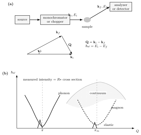
Top: a monochromator or chopper defines the incident state $(\mathbf k_i,E_i)$, and a detector or analyzer constrains $(\mathbf k_f,E_f)$ after scattering. The target receives $\mathbf Q=\mathbf k_i-\mathbf k_f$ and $\hbar\omega=E_i-E_f$. Bottom: a reduced $(Q,\omega)$ map can contain elastic Bragg weight, a nuclear one-phonon branch near $\boldsymbol\tau$, a magnetic one-magnon branch near $\boldsymbol\tau_m$, and broad continuum weight. Their displayed widths and intensities include instrumental resolution and channel-dependent matrix elements.

Modern instruments often save individual neutron events with:

$$\left( p, t_{\mathrm{det}}, t_{\mathrm{source}}, \Omega_{\mathrm{inst}}, \Omega_{\mathrm{sample}}, t_{\mathrm{run}} \right),$$

where $p$ labels a detector pixel, the times determine flight paths or pulse phase, and the angular coordinates specify instrument and sample orientation. Reactor instruments may instead accumulate counts directly at selected monochromator, sample, analyzer, and detector settings.

Metadata needed for a physical cross section include:

• source pulse or monitor counts and incident-spectrum calibration;
• flight-path lengths, chopper phases, monochromator and analyzer reflections;
• detector position, efficiency, dead time, masks, and time-independent background;
• sample orientation matrix, mass, composition, mosaic, shape, and environment;
• incident and final polarization efficiencies where applicable;
• empty-container, empty-instrument, vanadium, and transmission measurements;
• every rebinning, symmetry operation, merge, and background model.

The detector does not label an event “phonon” or “magnetic.” That label enters after coordinate conversion and cross-section comparison.

Scattering Kinematics

This page defines momentum and energy transferred to the sample as

$$\mathbf Q = \mathbf k_i-\mathbf k_f, \qquad \hbar\omega = E_i-E_f.$$

Positive $\omega$ means the neutron lost energy and created or excited something in the sample. Negative $\omega$ means the neutron gained energy by annihilating a thermally occupied excitation. Some diffraction and crystallography software uses the opposite sign for $\mathbf Q$; the intensity may look unchanged while complex structure factors and polarization conventions do not.

If $\phi$ is the angle between the incident and final wavevectors,

$$Q^2 = k_i^2+k_f^2 - 2k_i k_f\cos\phi.$$

For elastic scattering, $k_i=k_f=k$ and

$$Q = 2k \sin \left( \frac{\phi}{2} \right).$$

In a crystal, it is useful to decompose

$$\mathbf Q = \boldsymbol\tau+\mathbf q,$$

where $\boldsymbol\tau$ is a reciprocal-lattice vector and $\mathbf q$ lies in a chosen Brillouin zone. A magnetic structure can have a larger real-space unit cell and a different reciprocal vector $\boldsymbol\tau_m$. The instrument measures absolute $\mathbf Q$; reducing it into a chemical or magnetic zone is an analysis convention that must be stated.

Energy and momentum transfer are coupled by the neutron dispersion. At fixed $E_i$, not every desired $(\mathbf Q,\omega)$ point is reachable at every detector angle. Sample rotation, incident energy, analyzer setting, and scattering plane determine coverage. A visually empty region can be kinematically inaccessible rather than physically dark.

Elastic, Quasielastic, and Inelastic Scattering

Elastic diffraction

Elastic scattering has $\omega=0$ within resolution. Long-range periodic nuclear order produces Bragg peaks at reciprocal vectors. A nuclear unit-cell amplitude is

$$F_N(\mathbf Q) = \sum_d o_d b_d e^{-W_d(\mathbf Q)} e^{i\mathbf Q\cdot\mathbf r_d},$$

where $o_d$ is occupancy and $e^{-W_d}$ is the Debye–Waller amplitude. After Lorentz, multiplicity, absorption, extinction, preferred-orientation, and instrument corrections, integrated Bragg intensity constrains $\lvert F_N\rvert^2$.

Magnetic order similarly gives elastic peaks through a magnetic structure factor projected perpendicular to $\mathbf Q$. Magnetic peaks can occur at nuclear-forbidden positions or coincide with nuclear reflections. Their temperature dependence and decay with magnetic form factor help, but polarized analysis or a full magnetic refinement may be needed.

A Bragg peak establishes a nonzero spatial Fourier component averaged over the probe’s time window. It does not by itself identify the microscopic interaction that selected the order. Peak width constrains correlation length only after deconvolving instrument resolution, mosaic, strain, finite domain size, and sample-shape effects.

Quasielastic scattering

Slow fluctuations appear as intensity centered near $\omega=0$ with finite width. Diffusion, domain motion, spin relaxation, glassy dynamics, and rotational or translational molecular motion can all be quasielastic. If the intrinsic width is narrower than the instrument resolution, the signal is experimentally elastic even if the microscopic process is dynamic.

Backscattering and neutron spin echo access much slower timescales than conventional thermal-neutron spectroscopy. Comparing instruments therefore requires a time-window statement. “Static” means static on the stated resolution scale.

Inelastic scattering

Inelastic events have resolvable $\omega\ne0$. They can reveal:

• phonons and molecular vibrations through nuclear displacement correlations;
• magnons, paramagnons, and crystal-field transitions through magnetic correlations;
• diffusion and relaxational continua;
• multiphonon and multimagnon states;
• fractionalized or emergent-gauge continua;
• hybrid magnetoelastic modes containing both nuclear and magnetic weight.

Mode energy, intrinsic linewidth, and integrated spectral weight are distinct observables. A constant-$\mathbf Q$ scan, a constant-energy slice, and a cut following a dispersion convolve the four-dimensional resolution differently.

Dynamic Structure Factors and the Measured Cross Section

For a target operator $O_{\mathbf Q}$, a representative per-particle convention is

$$\begin{aligned} S_{OO}(\mathbf Q,\omega) &= \frac{1}{2\pi N} \int_{-\infty}^{\infty} dt\, \\ &\quad\times e^{i\omega t} \left\langle O_{\mathbf Q}(t) O_{-\mathbf Q}(0) \right\rangle. \end{aligned}$$

Density, isotope-weighted displacement, and magnetization operators define different structure factors. Structure Factors owns normalization changes, connected pieces, elastic delta functions, detailed balance, and response relations. A neutron paper must still state whether its horizontal energy coordinate is $\omega$ or $\hbar\omega$, whether intensity is per formula unit or magnetic ion, and which Cartesian components have been summed.

At thermal equilibrium,

$$S(\mathbf Q,-\omega) = e^{-\beta\hbar\omega} S(-\mathbf Q,\omega).$$

This detailed-balance relation is both physics and a diagnostic. Failure can signal an incorrect sign convention, temperature mismatch, background subtraction error, detector normalization problem, or genuine nonequilibrium.

The recorded intensity in bin $x$ is better represented schematically as

$$\begin{aligned} C(x) &= T_{\mathrm{run}} \int d\mathbf Q'\,d\omega' \\ &\quad\times \Phi\, \epsilon\, \mathcal A \\ &\quad\times R \left( x;\mathbf Q',\omega' \right) \\ &\quad\times \frac{d^2\sigma}{ d\Omega\,dE_f } \\ &\quad+ B(x). \end{aligned}$$

$\Phi$ is incident flux, $\epsilon$ detector efficiency, $\mathcal A$ sample transmission and attenuation, $R$ the resolution kernel, and $B$ background. Their arguments have been suppressed for readability. The resolution ellipsoid or volume can be tilted in $(\mathbf Q,\omega)$ space, so a steep dispersion can look broadened, split, or shifted. Fitting an unconvolved Lorentzian to such a cut does not generally recover a lifetime.

Instrument Architectures

Diffraction

A diffractometer emphasizes elastic intensity. Powder diffraction trades directional information for orientational averaging and broad reciprocal-space coverage. Single-crystal diffraction retains directions and domain information but requires an orientation model and adequate reciprocal-space sampling. Energy-integrating detectors can admit inelastic contamination; filters and wavelength discrimination matter.

Triple-axis spectroscopy

A triple-axis spectrometer uses:

1. a monochromator to select $\mathbf k_i$;
2. sample rotation and scattering angle to choose $\mathbf Q$;
3. an analyzer to select $\mathbf k_f$ before detection.

Holding $E_f$ fixed is common because it stabilizes analyzer and detector conditions, but fixed-$E_i$ operation is also possible. Triple-axis instruments make targeted trajectories through $(\mathbf Q,\omega)$ with tunable collimation and focusing. They are efficient when the expected signal is localized, and inefficient for discovering an unknown response over a large volume.

Higher-order wavelength contamination, monitor sensitivity, analyzer harmonics, focusing, and resolution geometry must be included. A scan coordinate is not necessarily orthogonal to a dispersing branch.

Time-of-flight spectroscopy

At a pulsed source, choppers select an incident-energy band and detector arrival times infer $E_f$. A direct-geometry instrument usually fixes $E_i$ and records broad angular and energy coverage simultaneously. Rotating a single crystal builds a four-dimensional dataset. Indirect-geometry instruments instead constrain $E_f$ with analyzer crystals.

Time-of-flight coverage is broad but highly nonuniform. Detector gaps, frame overlap, chopper transmission, incident flux, and the $k_f/k_i$ phase-space factor shape the raw map. Merging several $E_i$ settings can extend dynamic range only if their normalizations and resolutions are retained.

High-resolution and polarized methods

• Backscattering uses near-$180^\circ$ Bragg geometry for very fine energy resolution over a restricted range.
• Neutron spin echo encodes energy transfer in a Larmor phase and measures an intermediate scattering function over long times.
• Polarization analysis resolves spin-flip and non-spin-flip channels, magnetic components, and nuclear–magnetic interference.
• Small-angle scattering targets structures much larger than an atomic spacing near $Q=0$.
• Reflectometry resolves depth profiles normal to an interface under a layered optical model.

Instrument names are not interchangeable labels for $S(\mathbf Q,\omega)$. Each architecture samples and convolves a different region.

Phonons

For one-phonon coherent nuclear scattering at

$$\mathbf Q = \boldsymbol\tau+\mathbf q,$$

the mode-dependent amplitude contains

$$F_\nu(\mathbf Q) = \sum_d \frac{ b_d e^{-W_d(\mathbf Q)} }{ \sqrt{M_d} } \left[ \mathbf Q\cdot \mathbf e_{d\nu}(\mathbf q) \right] e^{i\mathbf Q\cdot\mathbf r_d}.$$

The corresponding creation intensity scales schematically as

$$I_\nu^{(+)} \propto \frac{k_f}{k_i} \frac{ \left| F_\nu(\mathbf Q) \right|^2 }{ \omega_\nu(\mathbf q) } \left[ n_{\mathrm B} \left( \omega_\nu \right) + 1 \right],$$

before multiphonon terms and resolution convolution.

This kernel explains why:

• a mode can disappear when $\mathbf Q\cdot\mathbf e_{d\nu}=0$;
• basis atoms interfere differently in different reciprocal zones;
• light atoms can have large displacement amplitudes;
• creation remains possible at zero temperature, while annihilation loses Bose population;
• phonon intensity often grows with $Q$ through the displacement factor even when a magnetic form factor is falling.

Measuring the same reduced $\mathbf q$ in several zones is therefore a polarization and eigenvector test, not redundant repetition. A fitted force-constant model should reproduce frequencies and absolute or consistently normalized intensities across zones. The Phonons page owns the dynamical matrix, branch structure, thermodynamics, and anharmonic interpretation.

Powder incoherent measurements can approximate a neutron-weighted vibrational density of states. The weights depend roughly on scattering cross section divided by mass, and multiphonon subtraction is model dependent. Calling the result “the phonon DOS” without its neutron weighting can mislead comparisons with calculations or other probes.

Magnons and Magnetic Excitations

A magnetic mode contributes through the same transverse projector and form factor that govern the general magnetic cross section. For a branch $\nu$, the intensity contains a matrix element of the magnetization operator,

$$\mathcal M_\nu^\alpha(\mathbf Q) = \left\langle \nu,\mathbf q \middle| M_{\mathbf Q}^\alpha \middle| 0 \right\rangle,$$

combined as

$$\sum_{\alpha,\beta} \left( \delta_{\alpha\beta} - \widehat Q_\alpha\widehat Q_\beta \right) \mathcal M_\nu^\alpha \mathcal M_\nu^{\beta *}.$$

Peak positions alone do not determine an exchange Hamiltonian. A credible spin-wave refinement predicts:

• the chemical and magnetic zone conventions;
• every branch and degeneracy;
• sublattice interference and polarization;
• domain populations and $g$-tensor anisotropy;
• magnetic-form-factor decay;
• field and temperature evolution;
• the resolution-convolved line shape.

Elastic magnetic diffraction should establish the reference structure before a harmonic magnon model is fitted. If the ordered state is not stationary under the proposed Hamiltonian, a numerically attractive dispersion fit is physically inconsistent. Spin Waves and Magnons develops that model-validation route.

At finite temperature or strong interaction, a magnon can shift, broaden, decay into several particles, or hybridize with a phonon. Avoided crossings accompanied by exchanged nuclear and magnetic intensity are stronger evidence for magnetoelastic hybridization than two nearby peak positions alone. Polarization analysis, reciprocal-zone dependence, field tuning, and isotope substitution can separate channels.

Magnetic absolute normalization enables moment sum-rule checks. In a common per-spin convention,

$$\frac{1}{N} \sum_{\mathbf q} \sum_\alpha \int_{-\infty}^{\infty} d\omega\, S^{\alpha\alpha}(\mathbf q,\omega) = S(S+1),$$

with prefactors adjusted to the stated Fourier convention and effective moment. Missing weight can lie outside the measured energy range, in an elastic contribution, in another polarization channel, or in degrees of freedom omitted by the model.

Spin-Liquid Continua

A local spin operator in a fractionalized phase can create two or more spinons or Majorana-like excitations. Their allowed total energies at fixed momentum fill a continuum rather than a single branch. Inelastic neutron scattering is therefore a natural probe of fractionalization.

The converse is false. Broad magnetic intensity can also arise from:

• two-magnon and higher-particle states;
• decay of a conventional mode into an allowed continuum;
• disorder-broadened local excitations or random singlets;
• overlapping crystal-field transitions;
• unresolved dispersive branches or domains;
• phonon and multiphonon backgrounds;
• multiple scattering and sample-environment subtraction errors.

A strong continuum analysis should:

1. establish magnetic character through polarization, form-factor decay, temperature, or field response;
2. map boundaries and internal structure over enough $(\mathbf Q,\omega)$ volume to test a microscopic model;
3. compare against conventional multiparticle, disorder, and crystal-field alternatives;
4. enforce detailed balance and an absolute spectral-weight sum rule;
5. vary resolution and incident energy to expose multiple scattering or unresolved modes;
6. combine with diffraction, local probes, thermodynamics, and heat transport to identify the phase.

The broad response measured in herbertsmithite is important fractionalization-compatible evidence, but defect Cu moments complicate the low-energy limit. The continuum in $\alpha$-RuCl$_3$ is consistent with proximity to Kitaev physics, while its zero-field ground state is magnetically ordered. A neutron continuum supports a dynamical account; it does not by itself measure topological order or identify the fractional quasiparticle uniquely. Quantum Spin Liquids owns that phase-level evidence ledger.

Resolution, Background, and Absolute Units

Resolution is multidimensional

Instrument resolution is a probability distribution in momentum and energy, not one scalar number. It depends on source pulse, chopper opening, monochromator and analyzer mosaic, collimation, detector geometry, sample mosaic and shape, and scan location. Report the resolution calculation or calibration at the relevant point.

For a Gaussian peak measured along a single cut, subtracting squared widths can be a useful approximation only when intrinsic and resolution profiles are both Gaussian and aligned with that cut. A Lorentzian lifetime convolved with a Gaussian resolution gives a Voigt-like profile. In either case, simulate the full dispersion within the multidimensional kernel when slopes are appreciable.

Background is a physical model

Common contributions include:

• empty cryostat, pressure-cell, magnet, and sample-can scattering;
• incoherent nuclear and isotope background;
• fast-neutron, gamma, electronic, and time-independent detector backgrounds;
• phonons beneath magnetic scattering and magnetic scattering beneath phonons;
• multiple scattering and aluminum powder rings;
• absorption, self-shielding, and wavelength-dependent transmission;
• sample holder, glue, grease, exchange gas, and contamination.

An empty-container run is not automatically the correct background because adding the sample changes attenuation and multiple scattering. High-temperature subtraction can remove magnetic spectral weight or alter phonons. Off-zone subtraction can fail when the background itself depends on $\mathbf Q$. State the model and test alternatives.

Normalization

Monitor normalization corrects source exposure but not every spectral or detector effect. Vanadium is commonly used because its strong incoherent scattering provides a nearly featureless detector-efficiency standard over appropriate conditions. Converting to absolute units additionally requires sample amount, attenuation, kinematic factors, and a cross-section convention.

Absolute normalization is especially valuable when comparing samples, enforcing moment or phonon sum rules, and claiming spectral-weight transfer. Arbitrary-color maps can establish a dispersion but cannot close a missing-weight argument.

Reproducible Workflow

Before beam time

1. Define the target operator and required $(\mathbf Q,\omega)$ region, not merely the material name.
2. Estimate scattering, incoherent, absorption, and transmission cross sections isotope by isotope.
3. Choose sample mass, shape, orientation, mosaic, and deuteration with the forward model in mind.
4. Simulate kinematic coverage and resolution for candidate instruments and incident energies.
5. Identify nuclear and magnetic reciprocal zones where the predicted polarization factors differ.
6. Plan empty-container, vanadium, transmission, background, and temperature or field controls.

During acquisition

• refine the orientation matrix using several noncoplanar reflections;
• monitor sample environment and beam stability continuously;
• acquire repeated reference cuts to catch sample motion or changing background;
• preserve event-mode data and run logs where available;
• measure more than one reciprocal zone for mode identification;
• collect both energy-loss and energy-gain sides when detailed balance is a useful check;
• avoid irreversible sample changes from heating, pressure cycling, field history, or radiation.

During reduction and fitting

1. Apply detector masks, calibration, monitor normalization, and coordinate conversion with versioned parameters.
2. Keep raw, corrected, background, and final intensity separately.
3. Propagate counting uncertainty through rebinning and subtraction; note induced covariance.
4. Record every symmetry fold and never use symmetrization as evidence of the symmetry imposed.
5. Fit a cross section convolved with resolution and integrated over the actual bin volume.
6. compare residuals in the full sampled space, not only along a favorable line.
7. archive orientation, sample, instrument, environment, reduction, and fitting files with the plotted data.

Common Artifacts and Failure Modes

Observation	Possible physics	Essential alternatives and checks
extra elastic peak	superstructure or magnetic order	multiple diffraction, contaminant phase, higher-order wavelength
broad elastic peak	short-range order or finite domains	instrument resolution, mosaic, strain, powder averaging
near-zero-energy wing	slow dynamics or diffusion	elastic-tail model, background, finite time window
missing phonon branch	polarization or basis extinction	kinematic gap, weak flux, wrong zone, overlapping mode
intensity falling with $Q$	magnetic form factor	absorption, detector efficiency, structure-factor cancellation
broad magnetic band	multiparticle or fractional continuum	disorder, crystal fields, phonons, unresolved branches, multiple scattering
apparent linewidth growth	intrinsic decay	tilted resolution ellipsoid, bin integration, mosaic, branch overlap
temperature-subtracted signal	changing magnetic response	Bose-populated phonons, Debye–Waller change, sample environment
spin-flip excess	magnetic scattering	imperfect polarization, guide-field errors, depolarization
absolute weight deficit	missing moment or itinerancy	unmeasured energy, elastic weight, form factor, normalization, absorption

Common Mistakes

• Treating counts as $S(\mathbf Q,\omega)$. Flux, efficiency, cross-section factors, attenuation, background, and resolution intervene.
• Leaving the transfer convention implicit. State whether $\mathbf Q=\mathbf k_i-\mathbf k_f$ and whether positive energy is transferred to the sample.
• Calling energy-integrated intensity elastic. It may include quasielastic or inelastic events inside the acceptance.
• Reading a missing mode as a missing excitation. Polarization, basis interference, form factor, and kinematic coverage can extinguish it.
• Fitting only peak centers. Intensities, widths, domains, and sum rules often discriminate models more strongly.
• Subtracting a high-temperature dataset without a Bose and Debye–Waller model. The subtraction can manufacture positive and negative features.
• Using one scalar resolution width. The relevant kernel is coupled in momentum and energy.
• Calling every broad magnetic response fractionalization. Conventional multiparticle, disorder, and instrumental explanations require explicit tests.
• Assuming deuteration changes only background. Isotope mass and chemistry can change the material response.
• Symmetrizing before testing symmetry. Preserve and show the unsymmetrized data.
• Claiming a bulk phase from one spectral feature. Combine the neutron result with static, local, thermodynamic, and transport evidence.

Connections

• Unconventional Superconductivity treats a superconductivity-induced spin resonance as one constraint on gap sign and representation, never proof by itself; this page retains calibrated and polarized dynamic-structure-factor extraction, resolution, and magnetic alternatives.
• Magnetic Moments in Matter compares elastic and inelastic magnetic weight only after this page’s form factor, cross section, absolute normalization, coverage, background, and resolution corrections are declared.
• How Quantum Matter Is Measured supplies the general record-to-claim, resolution, and uncertainty framework.
• Vortex Matter, Pinning, and Flux Flow interprets small-angle vortex-lattice peaks, widths, disorder, and field-history evolution as collective mixed-state evidence after this page’s cross-section, background, coverage, and resolution controls.
• Reciprocal Lattice fixes the diffraction and momentum-reduction geometry.
• Structure Factors gives the canonical correlation functions, detailed balance, and sum rules behind the cross sections.
• Charge and Spin Density Waves develops finite-wavevector order, satellites, correlation lengths, and multi-probe phase identification.
• Phonons develops the vibrational eigenproblem and the interpretation of measured frequencies, eigenvectors, and linewidths.
• Spin Waves and Magnons develops magnetic branch calculations, intensity validation, and exchange-parameter identifiability.
• Quantum Spin Liquids distinguishes continuum evidence from a complete fractionalized-phase claim.
• X-Ray Scattering provides the complementary electron-density, resonant, coherent, and small-sample photon probe.

References

1. L. Van Hove, “Correlations in Space and Time and Born Approximation Scattering in Systems of Interacting Particles”, Physical Review 95, 249–262 (1954).
2. C. G. Shull and J. S. Smart, “Detection of Antiferromagnetism by Neutron Diffraction”, Physical Review 76, 1256–1257 (1949).
3. B. N. Brockhouse, “Slow Neutron Spectroscopy and the Grand Atlas of the Physical World”, Reviews of Modern Physics 67, 735–746 (1995).
4. C. G. Shull, “Early Development of Neutron Scattering”, Reviews of Modern Physics 67, 753–757 (1995).
5. V. F. Sears, “Neutron Scattering Lengths and Cross Sections”, Neutron News 3(3), 26–37 (1992).
6. G. L. Squires, Introduction to the Theory of Thermal Neutron Scattering, 3rd ed., Cambridge University Press (2012).
7. S. W. Lovesey, Theory of Neutron Scattering from Condensed Matter, Clarendon Press (1984).
8. R. M. Moon, T. Riste, and W. C. Koehler, “Polarization Analysis of Thermal-Neutron Scattering”, Physical Review 181, 920–931 (1969).
9. M. J. Cooper and R. Nathans, “The Resolution Function in Neutron Diffractometry. I. The Resolution Function of a Neutron Diffractometer and Its Application to Phonon Measurements”, Acta Crystallographica 23, 357–367 (1967).
10. O. Arnold et al., “Mantid — Data Analysis and Visualization Package for Neutron Scattering and μSR Experiments”, Nuclear Instruments and Methods in Physics Research A 764, 156–166 (2014).
11. P. C. Hohenberg and W. F. Brinkman, “Sum Rules for the Frequency Spectrum of Linear Magnetic Chains”, Physical Review B 10, 128–131 (1974).
12. D. A. Tennant, R. A. Cowley, S. E. Nagler, and A. M. Tsvelik, “Measurement of the Spin-Excitation Continuum in One-Dimensional KCuF$_3$ Using Neutron Scattering”, Physical Review B 52, 13368–13380 (1995).
13. T.-H. Han et al., “Fractionalized Excitations in the Spin-Liquid State of a Kagome-Lattice Antiferromagnet”, Nature 492, 406–410 (2012).
14. A. Banerjee et al., “Proximate Kitaev Quantum Spin Liquid Behaviour in a Honeycomb Magnet”, Nature Materials 15, 733–740 (2016).
15. Institut Laue–Langevin, Neutron Data Booklet, 2nd ed. (2003).
16. National Institute of Standards and Technology Center for Neutron Research, “Neutron Scattering Lengths and Cross Sections”, isotope-resolved thermal-neutron tables.
17. Joint Committee for Guides in Metrology, Evaluation of Measurement Data — Guide to the Expression of Uncertainty in Measurement, JCGM 100:2008.

Exercises

Exercise 1: Wavelength and incident energy

A cold-neutron instrument selects $\lambda=4.00\,\mathrm{\mathring A}$. Find $k_i$ and $E_i$.

Solution

The wavevector magnitude is

$$\begin{aligned} k_i &= \frac{2\pi}{4.00\,\mathrm{\mathring A}} \\ &\simeq 1.571\,\mathrm{\mathring A}^{-1}. \end{aligned}$$

Using the wavelength conversion,

$$\begin{aligned} E_i &\simeq \frac{81.81}{ (4.00)^2 }\,\mathrm{meV} \\ &\simeq 5.11\,\mathrm{meV}. \end{aligned}$$

The wavelength and energy are not independent settings for a free neutron.

Exercise 2: Elastic scattering triangle

An elastic experiment has $k_i=k_f=2.50\,\mathrm{\mathring A}^{-1}$. The angle between $\mathbf k_i$ and $\mathbf k_f$ is $\phi=60^\circ$. Find $Q$.

Solution

For elastic scattering,

$$\begin{aligned} Q &= 2k \sin \left( \frac{\phi}{2} \right) \\ &= 2 \left( 2.50\,\mathrm{\mathring A}^{-1} \right) \sin30^\circ \\ &= 2.50\,\mathrm{\mathring A}^{-1}. \end{aligned}$$

The equality between $Q$ and $k$ is special to $\phi=60^\circ$; it is not a general elastic-scattering identity.

Exercise 3: Hydrogen and deuterium background

Using $\sigma_{\mathrm{inc}}(\mathrm H)=80.27$ barns and $\sigma_{\mathrm{inc}}(\mathrm D)=2.05$ barns, estimate the incoherent-background reduction per substituted nucleus when H is replaced by D. State one reason that the deuterated sample still requires independent characterization.

Solution

The cross-section ratio is

$$\frac{ \sigma_{\mathrm{inc}}(\mathrm H) }{ \sigma_{\mathrm{inc}}(\mathrm D) } = \frac{80.27}{2.05} \simeq 39.2.$$

The idealized incoherent contribution per substituted site is therefore reduced by about a factor of $39$. Deuterium changes the nuclear mass and zero-point motion; it can also change lattice constants, hydrogen bonding, exchange, transition temperatures, or phase stability. The deuterated material cannot be assumed identical apart from counting background.

Exercise 4: Detailed-balance ratio

For an excitation energy $\hbar\omega=5.0\,\mathrm{meV}$ at $T=50\,\mathrm K$, estimate the ratio $S(-\mathbf Q,-\omega)/S(\mathbf Q,\omega)$ assuming inversion-equivalent momenta. Use $k_{\mathrm B}=0.08617\,\mathrm{meV\,K^{-1}}$.

Solution

Detailed balance gives

$$\frac{ S(-\mathbf Q,-\omega) }{ S(\mathbf Q,\omega) } = \exp \left( -\frac{\hbar\omega}{k_{\mathrm B}T} \right).$$

Here

$$k_{\mathrm B}T = 0.08617\times50\,\mathrm{meV} \simeq 4.31\,\mathrm{meV},$$

so

$$\exp \left( -\frac{5.0}{4.31} \right) \simeq 0.313.$$

The neutron-energy-gain side should carry about $31\%$ of the corresponding loss-side intensity before asymmetric kinematic, detector, or background effects.

Exercise 5: A resolution-limited width

A Gaussian energy cut has measured FWHM $w_{\mathrm{obs}}=0.60\,\mathrm{meV}$. A calibration at the same kinematic point gives Gaussian resolution FWHM $w_R=0.40\,\mathrm{meV}$. Estimate the intrinsic Gaussian FWHM. Why should it not automatically be converted into a lifetime?

Solution

Aligned Gaussian variances add, and FWHM is proportional to the standard deviation. Therefore

$$\begin{aligned} w_{\mathrm{int}} &= \sqrt{ w_{\mathrm{obs}}^2-w_R^2 } \\ &= \sqrt{ (0.60)^2-(0.40)^2 }\,\mathrm{meV} \\ &\simeq 0.447\,\mathrm{meV}. \end{aligned}$$

This one-dimensional estimate assumes Gaussian intrinsic and resolution profiles with no dispersion crossing a tilted resolution volume. Exponential decay produces a Lorentzian spectral line, not a Gaussian one. A lifetime therefore requires a dynamical line-shape model and multidimensional resolution convolution.

Exercise 6: Audit a continuum claim

A candidate magnet shows no magnetic Bragg peak, and an unpolarized inelastic map contains broad intensity over $2$–$12\,\mathrm{meV}$. List a minimal set of additional tests before identifying spinons.

Solution

A minimal program should:

1. establish that the intensity is magnetic using polarization analysis, magnetic-form-factor decay, and field or temperature dependence;
2. repeat with different incident energies and resolution to test unresolved modes and multiple scattering;
3. map continuum boundaries and momentum structure rather than one integrated cut;
4. compare with multiphonon, multimagnon, crystal-field, disorder, and domain models;
5. normalize the spectral weight and test detailed balance and magnetic sum rules;
6. use local probes to exclude slow freezing or tiny static moments and use thermodynamics to account for the magnetic entropy;
7. test a phase-specific prediction under field, pressure, or controlled disorder.

The two original observations constrain ordinary order and reveal broad dynamics. They do not uniquely determine the quasiparticles or establish a quantum-spin-liquid phase.