Raman and Optical Spectroscopy

Raman spectroscopy measures the small energy difference between an incident photon and a scattered photon after the material is left in a different state. In a crystal, that final state need not be a molecular vibration. It can be a zone-center phonon, two magnons with nearly opposite momenta, a crystal-field excitation, an electronic particle-hole continuum, a superconducting pair-breaking excitation, or a collective mode. Incident and analyzed photon polarizations select symmetry channels, giving Raman scattering a form of momentum-space and operator selectivity even though visible photons transfer little crystal momentum.

That selectivity is conditional. The detected intensity also depends on laser energy, resonance, absorption depth, refractive index, crystal orientation, domains, numerical aperture, polarization leakage, spectrograph response, fluorescence, substrate interference, and laser-induced heating. A peak can establish an excitation energy in one optical channel; it does not automatically identify the microscopic mode or measure its unweighted density of states.

A useful evidence ladder is:

1. detector record: counts versus spectrograph pixel, acquisition time, incident power, sample position, and polarization configuration;
2. calibrated spectrum: Raman shift, instrument line shape, dark and cosmic-ray treatment, and relative spectral response;
3. channel-resolved intensity: corrected spectra in declared propagation and polarization geometries, with substrate and fluorescence models;
4. response inference: mode frequency and linewidth, symmetry tensor, Bose-corrected susceptibility, continuum, or resonance profile under a forward model;
5. material claim: structure, phase transition, coupling mechanism, magnetic excitation, superconducting gap anisotropy, strain, doping, layer number, or another property supported by controls and complementary probes.

Canonical Scope

This page is the canonical home for Raman and closely neighboring optical-spectroscopy practice in quantum matter. It owns crystal Raman tensors and laboratory geometries, point-group channel selection, phonon and magnetic Raman workflows, electronic Raman response, resonance and polarization systematics, micro-Raman mapping, and the special complications of thin and low-dimensional samples.

Raman Spectroscopy owns Raman-shift conventions, induced polarizability, the Kramers–Heisenberg–Dirac amplitude, Stokes and anti-Stokes factors, rotational Raman structure, molecular depolarization, and the ordinary instrument chain. Phonons owns lattice eigenvectors, branch counting, force constants, and vibrational thermodynamics. Spin Waves and Magnons owns magnetic mode calculations and Hamiltonian inference. Susceptibilities and Spectral Functions own the general many-body response and line-shape language.

Optical conductivity, the dielectric function, and low-energy electrodynamics have separate canonical homes in the response-and-optics chapter and the later terahertz and infrared probe page. They are distinguished here so that Raman intensity is not mislabeled as absorption, conductivity, or photoluminescence.

What Raman Measures in a Crystal

Energy and momentum transfer

Let the incident laser have angular frequency $\omega_L$ and wavevector $\mathbf k_i$, and let the detected photon have $\omega_s$ and $\mathbf k_s$. Use positive Raman loss

$$\Omega = \omega_L-\omega_s >0$$

for Stokes scattering, and define

$$\mathbf q = \mathbf k_i-\mathbf k_s.$$

Visible photon momenta are small compared with a typical Brillouin-zone dimension. Even in backscattering,

$$q_{\max} \simeq \frac{4\pi n}{\lambda_0},$$

where $\lambda_0$ is the vacuum wavelength and $n$ is the material refractive index. First-order Raman scattering therefore usually probes excitations near crystal momentum $\mathbf q=\mathbf0$, subject to refraction and finite optical penetration.

This does not limit every Raman feature to a zone-center elementary excitation. A two-particle process can create momenta $\mathbf k$ and $-\mathbf k+\mathbf q$ whose total matches the small photon transfer. Disorder, edges, superlattices, finite size, and double-resonant processes can also relax the elementary momentum selection.

Response-function form

After the intermediate electronic states are reduced to an effective material operator $\mathcal R_\gamma$, define

$$\chi_{\gamma\gamma}^{R}(t) = -i\theta(t) \left\langle \left[ \mathcal R_\gamma(t), \mathcal R_\gamma(0) \right] \right\rangle.$$

The label $\gamma$ contains the incident energy, polarizations, propagation geometry, and microscopic Raman vertex. A schematic Stokes intensity is

$$\begin{aligned} I_{\mathrm S}^{\mathrm{obs}}(\Omega) ={}& \int d\Omega'\, \mathcal G(\Omega-\Omega') C_\gamma(\Omega') \\ &\times \left[ 1+n_B(\Omega',T) \right] \chi_{\gamma\gamma}''(\Omega') +B(\Omega). \end{aligned}$$

$\mathcal G$ is the instrument line shape, $C_\gamma$ contains optical throughput and vertex factors, $n_B$ is the Bose function, and $B$ is background. The equation is a reduction, not a universal absolute cross section. Near electronic resonance, $C_\gamma$ can vary strongly across a Raman band and the effective-operator approximation may need to be replaced by the full intermediate-state amplitude.

The common Bose correction

$$\chi_{\gamma\gamma}''(\Omega) \propto \frac{ I_{\mathrm S}(\Omega) }{ 1+n_B(\Omega,T) }$$

is justified only after dark, response, background, and temperature-dependent optical factors are controlled. Dividing raw counts by $1+n_B$ does not remove fluorescence, resonant enhancement, or laser heating.

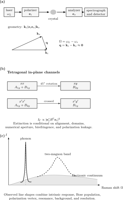
A material Raman experiment is specified by propagation and polarization vectors, not only by laser color. In a tetragonal in-plane example, parallel and crossed axes project different $A_{1g}$, $B_{1g}$, and $B_{2g}$ combinations. The measured spectrum can contain sharp lattice modes, broad magnetic weight, and an electronic continuum, all filtered by population, vertex, resonance, background, and resolution.

Raman Selection Rules in Materials

From the space group to the Raman tensor

At the Brillouin-zone center, a phonon transforms under an irreducible representation of the crystal little group. The leading electric-dipole Raman tensor is a derivative of the optical susceptibility with respect to the mode coordinate:

$$R_{ab}^{(\nu)} = \left. \frac{ \partial\chi_{ab}^{\mathrm{opt}} }{ \partial Q_\nu } \right|_{Q_\nu=0}.$$

The mode is Raman active when its representation occurs in the symmetric second-rank tensor built from electric-field components. Its intensity in an ideal fixed geometry is

$$I_\nu \propto \left| \mathbf e_s^* \cdot \mathbf R^{(\nu)} \cdot \mathbf e_i \right|^2.$$

Group theory determines allowed tensor components and exact zeros within a stated symmetry and operator approximation. It does not determine their numerical magnitudes, resonance profile, linewidth, or signal-to-background ratio.

The relevant symmetry is the actual ordered structure at the measurement temperature and field. A structural, magnetic, nematic, or charge-order transition can lower the point group, split degeneracies, activate folded modes, or mix tensors. Conversely, strain, defects, surfaces, and finite domains can produce weak nominally forbidden intensity without a bulk phase transition.

Tetragonal in-plane example

For a representative $D_{4h}$ crystal with axes $x$, $y$, and $z$, convenient symmetric tensors are

$$\begin{aligned} \mathbf R^{A_{1g}} &= \begin{pmatrix} a&0&0\\ 0&a&0\\ 0&0&b \end{pmatrix}, \\ \mathbf R^{B_{1g}} &= \begin{pmatrix} c&0&0\\ 0&-c&0\\ 0&0&0 \end{pmatrix}, \\ \mathbf R^{B_{2g}} &= \begin{pmatrix} 0&d&0\\ d&0&0\\ 0&0&0 \end{pmatrix}. \end{aligned}$$

For propagation near $z$ and in-plane linear polarization:

Geometry	Ideal symmetry content
$xx$	$A_{1g}+B_{1g}$
$xy$	$B_{2g}$
$x'x'$ with $x'=(x+y)/\sqrt2$	$A_{1g}+B_{2g}$
$x'y'$ with $y'=(x-y)/\sqrt2$	$B_{1g}$

These rows describe intensity channels, not coherent subtraction recipes. Extracting a “pure” response by subtracting spectra requires the relative optical throughput, tensor prefactors, and leakage to be calibrated.

Geometry must be reproducible

Porto notation writes a configuration as

$$\mathbf k_i \left( \mathbf e_i\mathbf e_s \right) \mathbf k_s.$$

For example, $z(xy)\bar z$ denotes backscattering along $z$, with incident polarization along $x$ and analyzed scattered polarization along $y$. A report should also state whether axes are laboratory, crystallographic, or sample-edge directions; how a miscut was measured; whether the analyzer was before or after a depolarizing optical element; and how the objective changes polarization.

Ideal extinction can be spoiled by:

• finite numerical aperture and longitudinal focal fields;
• birefringence and depth-dependent polarization;
• dichroism and different penetration depths for the two polarizations;
• objective, grating, mirror, and detector polarization response;
• imperfect polarizers and analyzer rotation offsets;
• twinning, rotational domains, mosaicity, and surface miscut;
• depolarization by roughness or multiple scattering.

Measure a leakage matrix with a known polarization state or reference crystal. A weak crossed-channel peak is evidence only after the expected leakage from a strong parallel-channel feature is propagated.

Phonons

First-order spectra probe the zone center

For a perfect crystal, first-order Raman scattering creates or annihilates one phonon with wavevector close to the photon transfer. Because $\mathbf q\approx\mathbf0$, it selects zone-center optical modes in an ordinary visible experiment. Acoustic modes approach zero frequency there and are usually studied by Brillouin scattering rather than a conventional Raman spectrograph.

The number and symmetry of Raman-active modes constrain the crystal structure. Useful signatures include:

• splitting of a degenerate representation under lowered symmetry;
• appearance of folded modes when a supercell forms;
• softening and linewidth growth near a structural instability;
• discontinuous frequency or intensity changes across a first-order transition;
• isotope shifts that test vibrational assignment;
• polarization rotation that identifies tensor components;
• spatial maps that reveal domains, strain, composition, or phase coexistence.

None is uniquely structural on its own. Electronic resonance can change intensity; strain can split modes; heating can soften them; and disorder can activate otherwise forbidden momentum.

Second-order and disorder-assisted features

Two-phonon Raman scattering can create phonons with approximately opposite momenta, so it samples weighted joint densities throughout the Brillouin zone. Defect-assisted processes can supply missing momentum. In graphene, the D band is defect activated, while the 2D band is a two-phonon double-resonant process that does not require a defect. These labels describe specific scattering pathways, not generic “first” and “second” overtones.

Assigning a broad band to a phonon density of states requires calculated dispersion, eigenvectors, resonance denominators, and matrix elements. A peak in a two-phonon spectrum can arise from a critical point, but its intensity is not the unweighted density of states.

Frequency, width, and Fano interference

An isolated damped phonon is often fitted with a Lorentzian or a resolution-convolved Voigt profile. Frequency shifts and linewidths can reflect thermal expansion, anharmonic decay, electron–phonon coupling, spin–phonon coupling, isotope disorder, strain distribution, or phase coexistence. A lifetime conversion must state whether the fit width is a half width or full width and whether the decay is amplitude or population.

If a discrete phonon interferes with a continuum, a Fano profile may be appropriate:

$$I(\epsilon) = I_0 \frac{ (q_F+\epsilon)^2 }{ 1+\epsilon^2 } +B,$$

where

$$\epsilon = \frac{\Omega-\Omega_0}{\Gamma}.$$

$q_F$ is an asymmetry parameter and $\Gamma$ is a convention-dependent scale. The sign of $q_F$ can reverse under a different definition of $\epsilon$. A good asymmetric fit supports interference but does not identify the continuum without independent evidence.

Thermometry and laser heating

Raman peak shifts, linewidths, and Stokes-to-anti-Stokes ratios can estimate temperature. Each is conditional:

• a frequency thermometer requires a phase- and strain-specific calibration;
• linewidth thermometry assumes the same decay channels;
• intensity-ratio thermometry requires relative spectral response, polarization, resonance, and the scattered-frequency factor;
• all three can disagree when optical and acoustic subsystems are out of equilibrium.

Measure spectra versus absorbed power, not only nominal power. Spot size, reflectance, substrate heat sinking, encapsulation, and environmental gas determine temperature rise. Extrapolation to zero power is often more trustworthy than declaring the lowest available power “nonheating.”

Magnons and Magnetic Continua

Visible photons carry little momentum, but exchange-mediated Raman scattering can create two magnetic excitations with nearly opposite momenta. For a Mott insulator with bond vectors $\mathbf d_{ij}$, a representative Fleury–Loudon operator is

$$\mathcal R_{\mathrm{FL}} = \sum_{\langle ij\rangle} \left( \mathbf e_i\cdot\mathbf d_{ij} \right) \left( \mathbf e_s^*\cdot\mathbf d_{ij} \right) J_{ij}\, \mathbf S_i\cdot\mathbf S_j.$$

The polarization dependence weights exchange bonds and transforms as a crystal symmetry channel. A two-magnon band can therefore sample exchange energies from across the magnetic Brillouin zone even though the total transferred momentum is nearly zero.

One-magnon Raman scattering is often forbidden in the simplest collinear, inversion-symmetric, spin-rotation-symmetric setting. It can become allowed through spin–orbit coupling, noncollinearity, magnetic dipole or antisymmetric vertices, resonance, broken inversion, or coupling to a phonon. The actual magnetic point group and microscopic light-coupling process decide the rule.

A magnetic Raman continuum may arise from:

• interacting or short-lived magnons;
• two- or multi-magnon states;
• spinons or other fractional excitations;
• disorder and random exchange;
• phonon or luminescence background;
• electronic particle-hole excitations.

Broad polarization-dependent weight that survives where phonons are excluded is valuable evidence, but it is not by itself a complete spin-liquid diagnosis. Compare field and temperature dependence, symmetry channels, energy sum scales, neutron spectra, thermodynamics, and a microscopic Raman operator.

Electronic Raman Response

Effective density vertex

In a nonresonant single-band effective-mass approximation, the electronic Raman operator can be written

$$\mathcal R_\gamma = \sum_{\mathbf k\sigma} \gamma_{\mathbf k}\, c_{\mathbf k\sigma}^\dagger c_{\mathbf k\sigma},$$

with vertex

$$\gamma_{\mathbf k} = \sum_{\alpha\beta} e_{s,\alpha}^* \frac{ \partial^2\varepsilon_{\mathbf k} }{ \partial k_\alpha\partial k_\beta } e_{i,\beta}.$$

This shows how polarization weights different regions of an anisotropic band. It is not exact in a multiband or resonant material: interband matrix elements, vertex corrections, spin–orbit coupling, and intermediate-state denominators can dominate.

For a tetragonal electronic structure, common basis functions are

$$\begin{aligned} \gamma_{B_{1g}}(\mathbf k) &\sim \cos k_x-\cos k_y, \\ \gamma_{B_{2g}}(\mathbf k) &\sim \sin k_x\sin k_y. \end{aligned}$$

In cuprate-like band structures these are often described as emphasizing antinodal and nodal sectors, respectively. That language is a material-dependent shorthand, not a universal theorem about the irrep labels.

Screening and the fully symmetric channel

Long-range Coulomb response can screen uniform charge fluctuations. In a simplified long-wavelength treatment, the screened Raman susceptibility has the structure

$$\chi_{\gamma\gamma}^{\mathrm{scr}} = \chi_{\gamma\gamma} - \frac{ \chi_{\gamma\rho} \chi_{\rho\gamma} }{ \chi_{\rho\rho} }.$$

The fully symmetric $A_{1g}$ channel is especially sensitive to charge backflow, multiband effects, and collective modes. Nonsymmetric channels can avoid part of this screening because their form factors average to zero by symmetry. Applying the scalar formula blindly to a layered, multiband, anisotropic, or resonant experiment is not justified.

What electronic features can mean

Electronic Raman spectra can show:

Feature	Candidate interpretation	Required caution
broad low-energy continuum	incoherent carriers, particle-hole excitations, or magnetic weight	fluorescence and luminescence subtraction
collision-dominated peak	symmetry-resolved electronic relaxation	vertex corrections and hydrodynamic limits
gap depletion and edge	density-wave, superconducting, or insulating gap	final-state interactions and momentum weighting
pair-breaking peak	superconducting quasiparticles in one symmetry channel	not generally equal to $2\Delta_{\max}$
sharp in-gap mode	exciton, amplitude mode, Leggett mode, or bound state	symmetry and many-body selection rules
quasielastic peak	slow order-parameter fluctuations	laser heating and central-Rayleigh tails

Raman response is a two-particle correlator. It is not the single-particle density of states measured by tunneling or photoemission, nor the current response measured by optical conductivity. Cross-probe comparison requires a common Hamiltonian with each probe’s vertex.

Resonance and Optical Complements

Resonant Raman scattering

When $\hbar\omega_L$ approaches an allowed electronic transition, one or more intermediate-state denominators become small. Intensities can increase dramatically and previously weak pathways can dominate. The Raman tensor then becomes complex and strongly dependent on incident energy, and the Placzek derivative picture may fail.

A resonance profile should be measured by changing laser energy while controlling:

• photon flux and focus;
• objective and grating throughput;
• penetration depth and optical interference;
• absorption and local heating;
• fluorescence background;
• detector response at the shifted wavelengths;
• sample position and damage history.

A peak that appears only at one laser energy may be resonantly enhanced rather than absent elsewhere. Conversely, destructive quantum interference can suppress a channel at a particular excitation energy.

Raman is not every optical spectrum

Method	Detector record	Leading material object
Raman scattering	photon counts versus energy loss	symmetry-resolved inelastic scattering response
absorption or transmission	removed or transmitted optical power	dielectric response plus propagation
reflectance	reflected power or field ratio	Fresnel response of surfaces and layer stack
ellipsometry	complex polarization ratio	model-dependent complex dielectric function
photoluminescence	spontaneous emission spectrum	occupied excited states, radiative matrix elements, and kinetics
optical conductivity	inferred complex current response	current-current susceptibility and diamagnetic term

Photoluminescence can overlap a Raman spectrum but has different laser-energy dependence: Raman features remain at approximately fixed shift, whereas fluorescence features often remain closer to fixed emission energy. This diagnostic is useful but not infallible near dispersive double-resonant features or strongly changing excitation profiles.

Reflectance, transmission, and ellipsometry can identify excitons, interband transitions, and absorption edges that explain a Raman resonance. Their inversion requires Fresnel or transfer-matrix modeling and, for conductivity, causality and sum-rule checks. They should constrain the Raman vertex rather than be relabeled as Raman data.

Low-Dimensional Materials

Micro-Raman spectroscopy is attractive for flakes and heterostructures because it is contactless, diffraction limited, and compatible with mapping. The small sample volume also magnifies optical and thermal systematics.

Substrate and layer-stack interference

The field at an atomically thin layer is the coherent sum of incident and reflected waves. The emitted Raman field also reflects and transmits through the stack. A measured band area therefore has the schematic form

$$I_{\mathrm{meas}} = \int dz\, \left| E_{\mathrm{exc}}(z) \right|^2 \left| E_{\mathrm{out}}(z) \right|^2 I_{\mathrm{int}}(z).$$

The enhancement depends on oxide thickness, refractive indices, numerical aperture, excitation wavelength, Raman shift, and layer position. Raw intensity ratios measured on different substrates are not intrinsic material ratios. A transfer-matrix calculation should use measured layer thicknesses and optical constants with uncertainty.

Graphene and related carbon systems

The G band is a zone-center optical phonon. The D band is defect activated through a double-resonant intervalley process. The 2D band is a two-phonon double-resonant feature and can be strong in clean material. Their positions, widths, shapes, dispersions with laser energy, and intensity ratios constrain layer structure, strain, doping, disorder, and electronic lifetime only through coupled models.

Correlated changes are more reliable than one empirical threshold. Strain and carrier density can both shift the G and 2D bands but along different trajectories in a calibrated two-frequency plot. Edge orientation, substrate interference, laser energy, and finite spot size must accompany any defect-density or layer-number inference.

Transition-metal dichalcogenides and heterostructures

In monolayer transition-metal dichalcogenides, reduced symmetry changes mode labels and optical selection rules. In-plane and out-of-plane phonons shift differently with layer number, strain, doping, dielectric environment, and temperature. Photoluminescence can reveal the crossover from an indirect bulk gap to a bright direct monolayer transition, while Raman constrains lattice symmetry and coupling.

Low-frequency shear and layer-breathing modes are especially sensitive to layer number, stacking, twist, and interlayer force constants. Folded phonons or moiré-activated features can indicate superlattice reconstruction, but contamination bubbles, strain gradients, rotational domains, and ordinary combination modes are alternatives.

For an anisotropic flake, record crystallographic orientation, edge assignment, incident and analyzed polarization, encapsulation, substrate, and transfer history. A polar plot without the optical-stack and birefringence model is not yet a Raman tensor.

Instrument, Calibration, and Mapping

Minimal material microscope

A typical micro-Raman system contains a narrow-line laser, cleanup filter, power control, polarization optics, microscope objective, sample stage and environment, Rayleigh-rejection filters, analyzer, spectrograph, and CCD or array detector. Low-frequency measurements may use volume Bragg gratings, multiple subtractive stages, or specialized interferometers.

Four calibrations are distinct:

1. shift calibration: maps detector pixel to Raman shift using known laser and reference lines;
2. resolution calibration: measures the instrument line shape and its dependence on slit, grating, wavelength, and pixel position;
3. relative-intensity calibration: measures wavelength-dependent throughput from sample plane to detector;
4. polarization calibration: measures preparation, leakage, and detection efficiency for each channel.

A silicon peak at the expected shift validates part of the first calibration. It does not establish intensity response, low-frequency rejection, or polarization purity.

Spatial maps are sampled fields

Raman maps report a fitted quantity at each focus position. The optical point-spread function, sample topography, stage drift, finite integration time, and fit covariance determine the true spatial resolution. A map pixel can be smaller than the diffraction-limited spot without providing independent subspot information.

Store spectra, not only peak-fit maps. A peak-tracking algorithm can exchange labels at crossings, lock onto fluorescence ripples, or convert a two-phase mixture into one broadened peak. Inspect residuals and representative raw spectra from every inferred region.

Laser dose is part of the sample state

Report wavelength, power at the sample, spot estimate, dwell, repetitions, scan order, and atmosphere. Compare:

• increasing and decreasing power;
• first and repeated exposure at one point;
• fresh and previously illuminated positions;
• continuous and chopped illumination where possible;
• Raman thermometry with an independent structural or optical stability marker.

Photo-oxidation, desorption, defect creation, phase transformation, and charge trapping can be irreversible. A spectrum recorded after damage is reproducible only as a damaged-state measurement.

Data Reduction and Forward Modeling

A detector bin $i$ can be represented as

$$\begin{aligned} d_i ={}& \int d\Omega\, R_i(\Omega) \eta_i(\Omega,\mathbf e_s) I_{\mathrm{sample}}(\Omega) \\ &+ F_i +D_i +C_i +\epsilon_i, \end{aligned}$$

where $R_i$ is spectral resolution and sampling, $\eta_i$ is throughput, $F_i$ is fluorescence or broad luminescence, $D_i$ is dark and fixed-pattern response, $C_i$ represents sparse cosmic-ray events, and $\epsilon_i$ is counting and read noise.

Baselines can remove physics

Polynomial, spline, penalized, and morphology-based baselines encode different smoothness assumptions. A broad electronic continuum, two-magnon band, or quasielastic response can be smoother than the chosen baseline and disappear into it. Publish raw and corrected spectra, baseline parameters, excluded regions, and sensitivity to a reasonable family of backgrounds.

Fluorescence is not always a smooth polynomial. It can contain vibronic structure, detector etaloning, or laser-dependent decay. Changing excitation wavelength, time gating, or using anti-Stokes data can provide stronger discrimination than a higher-order fit.

Fit area, width, and covariance together

Peak height is highly correlated with width and background. For overlapping modes, fit all spectra in a temperature, polarization, or spatial series with shared physical constraints when justified, while allowing enough flexibility to expose model failure. Report integrated area, peak position, width convention, covariance, instrument convolution, and residuals.

Do not convert a fitted Lorentzian width to a lifetime when inhomogeneous strain, unresolved splitting, spectral diffusion, or instrumental broadening dominates. A narrow peak can be resolution limited, and a broad peak can be a mixture rather than a short-lived quasiparticle.

What the Probe Can Establish

Observation	Defensible direct statement	Additional evidence needed
polarization extinction	weak response in a calibrated geometry	point-group assignment and leakage model
phonon splitting	more than one lattice component is resolved	structural symmetry, domains, or strain mechanism
soft mode	restoring scale decreases in one channel	thermodynamic transition and order parameter
two-magnon band	magnetic multi-particle Raman weight	exchange model and cross-probe spin spectrum
electronic continuum	inelastic weight beyond assigned phonons	fluorescence, luminescence, and magnetic separation
superconducting redistribution	response changes below $T_c$ in one vertex	gap model, screening, final-state effects, bulk confirmation
resonant enhancement	intermediate electronic states amplify a channel	excitation profile and absorption/heating controls
flake peak shift	local vibrational energy changes	separation of strain, doping, temperature, layer, and substrate

Common Mistakes

• Using molecular Raman selection rules without the crystal space group and measurement geometry.
• Calling every visible photon-scattering feature a zone-center phonon.
• Treating a two-phonon band as an unweighted phonon density of states.
• Assigning a weak crossed-polarization peak without measuring leakage.
• Comparing raw intensities across gratings, objectives, laser colors, or substrates.
• Bose-correcting raw counts before background and response correction.
• Calling an asymmetric phonon proof of electron–phonon coupling without identifying the continuum.
• Interpreting every broad magnetic continuum as fractionalization.
• Equating electronic Raman intensity with a single-particle density of states or optical conductivity.
• Reading a pair-breaking peak as exactly $2\Delta$ without vertex and final-state modeling.
• Inferring layer number from one empirical peak ratio outside its calibration domain.
• Calling map pixel spacing spatial resolution.
• Removing a broad continuum with a polynomial baseline and then claiming it is absent.
• Ignoring laser dose because the nominal power appears small.

A Reproducible Workflow

1. Define the target channel. State whether the goal is phonon symmetry, magnetic scattering, electronic response, resonance, mapping, or a low-dimensional material parameter.
2. Fix coordinates and symmetry. Record crystal axes, surface normal, domains, point group, and Porto geometry.
3. Choose the laser deliberately. Consider resonance, penetration, fluorescence, diffraction-limited spot, substrate interference, detector range, and damage.
4. Calibrate four axes. Validate shift, resolution, relative intensity, and polarization separately.
5. Measure controls. Acquire substrate, empty region, dark, reference, power series, repeat exposure, and alternative polarization or laser energy as appropriate.
6. Preserve raw spectra. Keep counts, acquisition metadata, masks, cosmic-ray flags, and scan order before baseline or fitting.
7. Fit the forward model. Include resolution, response, background, Bose factor, optical stack, and symmetry vertex at the level required by the claim.
8. Test alternatives. Vary baseline, line shape, leakage, temperature calibration, and mode assignment; inspect residuals and parameter covariance.
9. Compare orthogonal probes. Use diffraction for structure, neutron or RIXS for spin dynamics, transport for mobile carriers, and reflectance or ellipsometry for electronic resonances.
10. Report the inference boundary. Separate measured shift and polarization from the model-dependent material parameter.

Exercises

1. Why first-order Raman is near the zone center

A backscattering experiment uses vacuum wavelength $\lambda_0=532\ \mathrm{nm}$. Neglect refraction and estimate the maximum photon momentum transfer in $\mathrm{\mathring A}^{-1}$. Compare it with a typical Brillouin-zone scale of $1\ \mathrm{\mathring A}^{-1}$.

Solution

In backscattering,

$$q_{\max} = \frac{4\pi}{\lambda_0}.$$

Since $532\ \mathrm{nm}=5320\ \mathrm{\mathring A}$,

$$q_{\max} = \frac{4\pi}{5320\ \mathrm{\mathring A}} \simeq 2.36\times10^{-3}\ \mathrm{\mathring A}^{-1}.$$

This is about $0.24\%$ of a $1\ \mathrm{\mathring A}^{-1}$ zone scale. Refraction can multiply it by an index of order unity, but the first-order process still probes close to $\Gamma$. Two-particle, defect-assisted, or resonant processes can sample larger internal momenta while conserving the small total transfer.

2. Tetragonal polarization channels

Using the $D_{4h}$ tensors above, show that $xy$ selects $B_{2g}$ and $x'y'$ selects $B_{1g}$, where $x'=(x+y)/\sqrt2$ and $y'=(x-y)/\sqrt2$.

Solution

For $xy$ geometry,

$$\mathbf e_s^{\mathsf T} \mathbf R \mathbf e_i = R_{yx}.$$

Only $\mathbf R^{B_{2g}}$ has a nonzero $yx$ element, equal to $d$. The $A_{1g}$ and $B_{1g}$ tensors are diagonal.

For crossed rotated axes,

$$\begin{aligned} x'^{\mathsf T} \mathbf R^{B_{1g}} y' &= c, \\ x'^{\mathsf T} \mathbf R^{A_{1g}} y' &= 0, \\ x'^{\mathsf T} \mathbf R^{B_{2g}} y' &= 0. \end{aligned}$$

Thus ideal $x'y'$ isolates $B_{1g}$. In an experiment, finite leakage and domains set a nonzero extinction floor.

3. Bose population in a Stokes spectrum

A mode has Raman shift $100\ \mathrm{cm}^{-1}$, corresponding to $12.40\ \mathrm{meV}$. Assuming its intrinsic $\chi''$ and optical prefactor do not change, estimate the ratio of Stokes intensities at $300\ \mathrm K$ and $30\ \mathrm K$.

Solution

The Stokes population factor is

$$1+n_B = \frac{1}{ 1-e^{-\hbar\Omega/(k_BT)} }.$$

At $300\ \mathrm K$, $k_BT\simeq25.85\ \mathrm{meV}$, so

$$1+n_B(300\ \mathrm K) \simeq \frac{1}{1-e^{-12.40/25.85}} \simeq 2.63.$$

At $30\ \mathrm K$, $k_BT\simeq2.585\ \mathrm{meV}$:

$$1+n_B(30\ \mathrm K) \simeq 1.008.$$

Therefore

$$\frac{I_{\mathrm S}(300\ \mathrm K)}{ I_{\mathrm S}(30\ \mathrm K)} \simeq 2.61.$$

Real phonon frequency, linewidth, Raman tensor, absorption, and sample temperature can all change, so this is only the population contribution.

4. Fleury–Loudon selection on a square lattice

For a nearest-neighbor square-lattice Heisenberg model with equal bond length, evaluate the polarization weights in $x'y'$ geometry. Show why the resulting operator has $B_{1g}$ bond symmetry.

Solution

Take

$$\mathbf e_i=x' = \frac{x+y}{\sqrt2}, \qquad \mathbf e_s=y' = \frac{x-y}{\sqrt2}.$$

For an $x$ bond,

$$\left( \mathbf e_i\cdot x \right) \left( \mathbf e_s\cdot x \right) = \frac12.$$

For a $y$ bond, the product is $-1/2$. Hence

$$\mathcal R_{x'y'} \propto \frac{J}{2} \left[ \sum_{\langle ij\rangle_x} \mathbf S_i\cdot\mathbf S_j - \sum_{\langle ij\rangle_y} \mathbf S_i\cdot\mathbf S_j \right].$$

The sign changes under a $90^\circ$ rotation, which is the $B_{1g}$ bond pattern. The operator can create two-magnon weight even though the total photon momentum is small.

5. A Fano zero and maximum

For the normalized Fano factor

$$f(\epsilon) = \frac{(q_F+\epsilon)^2}{1+\epsilon^2},$$

take $q_F=2$. Find the antiresonance zero and the finite stationary maximum.

Solution

The numerator vanishes at

$$\epsilon=-q_F=-2.$$

Differentiating gives stationary points at $\epsilon=-q_F$ and

$$\epsilon = \frac{1}{q_F} = \frac12.$$

At the latter,

$$f\left(\frac12\right) = \frac{(2+1/2)^2}{1+(1/2)^2} = 5.$$

The asymmetric maximum and zero arise from interference. Changing the sign convention for $\epsilon$ changes the reported sign of $q_F$.

6. Substrate interference correction

Two nominally identical monolayers are measured on different optical stacks. The raw area of one Raman band is three times larger on stack A than on stack B. A transfer-matrix calculation predicts enhancement factors $F_A=4.0$ and $F_B=1.0$. What is the inferred intrinsic area ratio?

Solution

Write $I_{\mathrm{meas}}=F I_{\mathrm{int}}$. Then

$$\frac{ I_{\mathrm{int},A} }{ I_{\mathrm{int},B} } = \frac{ I_{\mathrm{meas},A}/F_A }{ I_{\mathrm{meas},B}/F_B } = \frac{3}{4} = 0.75.$$

The sample with the larger raw signal has the smaller inferred intrinsic area in this example. The numerical conclusion inherits uncertainty in thicknesses, optical constants, focus, and collection geometry.

Research Status

• Established: crystal Raman tensors, point-group selection rules, first-order zone-center phonon scattering, multiphonon processes, Fleury–Loudon magnetic scattering in its domain, electronic Raman susceptibilities, Bose population factors, and resonant intermediate-state effects.
• Model dependent: extracting electron–phonon coupling from a Fano profile, converting pair-breaking peaks to gap amplitudes, assigning continua to fractional excitations, inferring absolute strain or doping from empirical shifts, and recovering intrinsic intensity from a thin-film optical stack.
• Active: Raman vertices in multiorbital and spin–orbit-coupled materials, moiré-activated modes, nonequilibrium and ultrafast Raman response, quantum-light Raman protocols, nanoscale near-field Raman, and uncertainty-aware hyperspectral inversion.

Cross-Links

• Unconventional Superconductivity uses polarization-resolved pair-breaking and collective features as one constraint in a multi-probe pairing audit; this page retains Raman selection rules, resonance, backgrounds, and instrument inversion.
• Raman Spectroscopy gives the canonical Raman-shift, molecular polarizability, Stokes and anti-Stokes, and intermediate-state foundations.
• How Quantum Matter Is Measured supplies the general record-to-response-to-claim framework.
• Phonons owns lattice dynamics, polarization vectors, thermodynamics, and phonon lifetimes.
• Spin Waves and Magnons owns magnetic modes, exchange Hamiltonians, and cross-probe validation.
• Structure Factors explains why probe vertices and correlation functions must be distinguished.
• Susceptibilities develops retarded response channels and dissipation.
• Spectral Functions owns peaks, continua, linewidths, and resolution-aware interpretation.
• Kubo Formula derives causal linear response and optical conductivity.
• Drude Theory owns intraband optical conductivity and responsible electrodynamic fitting.
• Terahertz and Infrared Probes owns field-resolved low-energy conductivity, superconducting missing-area tests, polar phonons, and thin-film electrodynamic inversion.
• Low-Dimensional Quantum Matter develops dimensional crossover and the physical meaning of a low-dimensional material.
• Graphene owns graphene’s band, pseudospin, transport, strain-gauge, and correlated-state physics.

References

1. R. Loudon, “The Raman Effect in Crystals,” Advances in Physics 13, 423–482 (1964), doi:10.1080/00018736400101051.
2. W. Hayes and R. Loudon, Scattering of Light by Crystals (Wiley, 1978; Dover reprint, 2012).
3. M. Cardona, ed., Light Scattering in Solids I (Springer, 1975), doi:10.1007/978-3-540-37568-5.
4. D. L. Rousseau, R. P. Bauman, and S. P. S. Porto, “Normal Mode Determination in Crystals,” Journal of Raman Spectroscopy 10, 253–290 (1981), doi:10.1002/jrs.1250100152.
5. T. P. Devereaux and R. Hackl, “Inelastic Light Scattering from Correlated Electrons,” Reviews of Modern Physics 79, 175–233 (2007), doi:10.1103/RevModPhys.79.175.
6. P. A. Fleury and R. Loudon, “Scattering of Light by One- and Two-Magnon Excitations,” Physical Review 166, 514–530 (1968), doi:10.1103/PhysRev.166.514.
7. B. S. Shastry and B. I. Shraiman, “Theory of Raman Scattering in Mott–Hubbard Systems,” Physical Review Letters 65, 1068–1071 (1990), doi:10.1103/PhysRevLett.65.1068.
8. U. Fano, “Effects of Configuration Interaction on Intensities and Phase Shifts,” Physical Review 124, 1866–1878 (1961), doi:10.1103/PhysRev.124.1866.
9. M. Balkanski, R. F. Wallis, and E. Haro, “Anharmonic Effects in Light Scattering Due to Optical Phonons in Silicon,” Physical Review B 28, 1928–1934 (1983), doi:10.1103/PhysRevB.28.1928.
10. C. Kranert, C. Sturm, R. Schmidt-Grund, and M. Grundmann, “Raman Tensor Formalism for Optically Anisotropic Crystals,” Physical Review Letters 116, 127401 (2016), doi:10.1103/PhysRevLett.116.127401.
11. A. C. Ferrari and D. M. Basko, “Raman Spectroscopy as a Versatile Tool for Studying the Properties of Graphene,” Nature Nanotechnology 8, 235–246 (2013), doi:10.1038/nnano.2013.46.
12. D. Yoon et al., “Interference Effect on Raman Spectrum of Graphene on SiO$_2$/Si,” Physical Review B 80, 125422 (2009), doi:10.1103/PhysRevB.80.125422.
13. C. Lee et al., “Anomalous Lattice Vibrations of Single- and Few-Layer MoS$_2$,” ACS Nano 4, 2695–2700 (2010), doi:10.1021/nn1003937.
14. K. F. Mak, C. Lee, J. Hone, J. Shan, and T. F. Heinz, “Atomically Thin MoS$_2$: A New Direct-Gap Semiconductor,” Physical Review Letters 105, 136805 (2010), doi:10.1103/PhysRevLett.105.136805.
15. P.-H. Tan, ed., Raman Spectroscopy of Two-Dimensional Materials (Springer, 2019), doi:10.1007/978-981-13-1828-3.
16. National Institute of Standards and Technology, “Relative Intensity Correction Standards for Fluorescence and Raman Spectroscopy”, including SRM 2241–2243 and related certificates.
17. A. Urbas, K. Gierz, and D. D. Leber, Certification of Standard Reference Material 2246a: Relative Intensity Correction Standard for Raman Spectroscopy, 830 nm Excitation, NIST SP 260-244 (2024), doi:10.6028/NIST.SP.260-244.
18. Joint Committee for Guides in Metrology, Evaluation of Measurement Data — Guide to the Expression of Uncertainty in Measurement, JCGM 100:2008.