Angle-Resolved Photoemission Spectroscopy

Angle-resolved photoemission spectroscopy, or ARPES, illuminates a surface with photons and measures the kinetic energy and emission direction of each detected electron. With a crystal orientation, photon energy, polarization, work-function convention, and final-state model, those detector coordinates can be converted into a binding energy and crystal momentum. Repeating the measurement builds an occupied energy–momentum intensity map.

The word measures needs care. ARPES does not photograph a pre-existing band structure. A photon removes an electron from an interacting $N$-electron state, the photoelectron propagates through the material and surface, and an analyzer accepts only part of the outgoing distribution. The measured counts combine removal spectral weight, occupation, dipole matrix elements, final-state propagation, escape depth, detector acceptance, background, and resolution.

A useful evidence ladder is:

1. detector record: counts versus kinetic energy, emission angles, photon setting, and time;
2. calibrated coordinates: binding energy and momentum under declared kinematic conventions;
3. intensity map: normalized counts with resolution, background, and processing recorded;
4. spectral inference: dispersions, linewidths, gaps, and spectral-weight changes under a forward model;
5. electronic-structure claim: band assignment, self-energy, symmetry breaking, surface state, or topology tested across photon energy, polarization, temperature, and independent probes.

A bright ridge can be highly informative. It is not, by itself, a complete band inventory or a direct many-body spectral function.

Canonical Scope

This page is the canonical home for solid-state ARPES practice: analyzer kinematics, energy and momentum calibration, instrumental and thermal resolution, the photoemission forward model, energy- and momentum-distribution curves, Fermi-surface and band mapping, out-of-plane momentum scans, surface sensitivity, matrix-element effects, correlation signatures, uncertainty, and reproducible reporting.

Photoelectron Spectroscopy owns general photoionization channels, binding-energy conventions, Dyson orbitals, angular distributions, and continuum scattering for atoms, molecules, and solids. Spectral Functions owns removal and addition spectral measures, self-energy line shapes, residues, sum rules, and lifetime conventions. Fermi Surface owns Bloch-band Fermi-surface geometry. This page connects those objects to a momentum-resolved solid-state experiment without duplicating their full derivations.

Conventional equilibrium ARPES is the focus. Spin-resolved, nano-ARPES, standing-wave, soft-x-ray, and time-resolved variants are introduced only where they change the inference. Pump–Probe Spectroscopy owns nonequilibrium preparation, finite probe-window interpretation, and population dynamics.

What the Apparatus Records

An ARPES experiment combines:

• a photon source with known energy $h\nu$, bandwidth, wavevector $\mathbf q_\gamma$, and polarization $\boldsymbol\epsilon$;
• an oriented sample in ultrahigh vacuum, often cleaved or grown in situ;
• an electrostatic analyzer that disperses electrons by kinetic energy;
• angular imaging or deflection optics that encode one or two emission angles;
• a detector whose pixels, gain, dead time, and nonlinearities must be calibrated.

The minimally useful raw event coordinates are

$$\left( E_{\mathrm{kin}}, \theta, \varphi, h\nu, \boldsymbol\epsilon, t \right),$$

supplemented by temperature, sample azimuth and tilt, photon flux, spot position, and preparation history. Here $\theta$ is measured from the surface normal and $\varphi$ is the in-plane azimuth under a declared geometry.

The familiar three-step description separates:

1. optical excitation inside the solid;
2. propagation of the excited electron toward the surface;
3. transmission through the surface barrier into vacuum.

This separation is a useful experimental ledger, not an exact factorization. One-step photoemission theory treats excitation, surface scattering, and escape coherently, with a time-reversed low-energy-electron-diffraction-like final state. Final-state diffraction and interference can therefore create structure that a plane-wave or three-step picture misses.

Energy and Momentum Kinematics

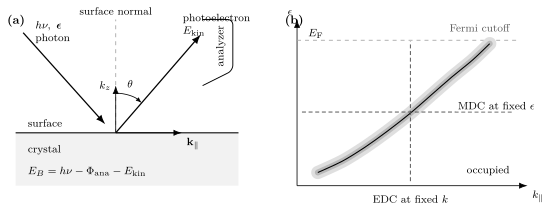
Left: a photon of energy $h\nu$ and polarization $\boldsymbol\epsilon$ ejects an electron with kinetic energy $E_{\mathrm{kin}}$ at polar angle $\theta$; the surface preserves parallel momentum modulo a surface reciprocal vector. Right: an ARPES map is measured intensity, not a bare dispersion. A vertical energy-distribution curve holds $\mathbf k$ fixed, while a horizontal momentum-distribution curve holds energy fixed.

Binding energy

For a conducting sample electrically connected to the analyzer, the Fermi levels equilibrate. A common analyzer-referenced ledger is

$$E_B = h\nu - \Phi_{\mathrm{ana}} - E_{\mathrm{kin}},$$

where $E_B\geq0$ denotes occupied-state binding energy below the Fermi level and $\Phi_{\mathrm{ana}}$ is the calibrated analyzer work function. If the intrinsic energy variable is measured relative to the chemical potential, this page uses

$$\epsilon = -E_B, \qquad \epsilon=0 \quad\text{at}\quad E_{\mathrm F}.$$

The sample work function controls the vacuum-level offset and low-energy cutoff, but it does not simply replace the analyzer work function in a Fermi-referenced spectrum when sample and analyzer are in good electrical contact. Contact potentials are handled by calibration. An insulating, poorly grounded, or photocharged sample can shift and broaden spectra in a flux-, time-, and position-dependent way, invalidating the simple ledger.

The energy zero should be checked against a metallic reference in electrical contact, commonly a clean polycrystalline metal. Report photon energy, reference temperature, fit model, drift, and whether sample and reference were measured simultaneously or sequentially.

Vacuum momentum

Outside the sample, the electron wavevector magnitude is

$$K = \frac{\sqrt{2m_eE_{\mathrm{kin}}}}{\hbar}.$$

A useful numerical conversion is

$$K\,[\text{\AA}^{-1}] \approx 0.512 \sqrt{ E_{\mathrm{kin}}\,[\mathrm{eV}] }.$$

Its surface-parallel components are

$$\mathbf K_\parallel = K\sin\theta \left( \cos\varphi, \sin\varphi \right).$$

Translational symmetry parallel to an ordered surface gives

$$\mathbf k_{i,\parallel} \equiv \mathbf K_\parallel - \mathbf q_{\gamma,\parallel} \pmod{\mathbf G_\parallel},$$

where $\mathbf k_i$ is the initial-state crystal momentum and $\mathbf G_\parallel$ is a surface reciprocal-lattice vector. In vacuum-ultraviolet ARPES, photon momentum is often small compared with a Brillouin-zone dimension, but it should not be silently neglected in soft-x-ray measurements or precision comparisons.

The analyzer reports laboratory angles. Converting them to $\mathbf k_\parallel$ requires the sample normal, azimuth, manipulator offsets, lens mode, detector distortion, and photon-incidence geometry. A high-symmetry cut is a conclusion of that calibration, not merely a manipulator readout.

Out-of-plane momentum

The surface breaks translation symmetry normal to itself, so $k_z$ is not exactly conserved. A commonly used free-electron final-state estimate is

$$\begin{aligned} k_z \approx{}& \frac{1}{\hbar} \sqrt{ 2m_e \left( E_{\mathrm{kin}}\cos^2\theta + V_0 \right) } \\ &- q_{\gamma,z} \pmod{G_z}, \end{aligned}$$

where $V_0$ is an empirical inner potential. This formula is a model, not a calibration identity. Real final states have band gaps, diffraction, self-energy broadening, and surface matching.

Photon-energy scans can identify periodic dispersion in $k_z$ and fit $V_0$, especially when symmetry planes repeat with the expected reciprocal period. Intensity variation with photon energy alone is insufficient because atomic cross sections and final-state matrix elements also vary strongly.

Finite escape depth $\lambda$ produces an intrinsic spread of normal momentum of order

$$\Delta k_z \sim \frac{1}{\lambda}.$$

A quasi-two-dimensional state can therefore look sharp in $k_z$, while a three-dimensional band is averaged over a finite slab of reciprocal space.

Resolution and Acceptance

Energy resolution

If independent photon and analyzer responses are approximately Gaussian, their full widths can be combined schematically as

$$\begin{aligned} \left( \Delta E_{\mathrm{inst}} \right)^2 &\approx \left( \Delta E_\gamma \right)^2 \\ &\quad+ \left( \Delta E_{\mathrm{ana}} \right)^2 \\ &\quad+ \left( \Delta E_{\mathrm{stab}} \right)^2. \end{aligned}$$

$\Delta E_{\mathrm{stab}}$ collects electrical noise, drift, and other approximately Gaussian contributions. This quadrature rule does not apply unchanged to asymmetric analyzer response, space-charge tails, or non-Gaussian source spectra.

Temperature broadens the occupied cutoff even for perfect instrumentation. The derivative of a Fermi function has full width at half maximum

$$\Delta E_T \approx 3.53\,k_{\mathrm B}T.$$

The observed Fermi edge is a convolution of this thermal form with the instrumental response. Treating its fitted width as purely instrumental overestimates the analyzer width.

Resolution trades against count rate. Narrow slits, low pass energy, small angular acceptance, and narrow photon bandwidth improve nominal resolution but reduce signal. High photon flux can introduce photoelectron space charge, shifting and broadening the spectrum. A flux series is needed to establish a space-charge-free operating regime.

Momentum resolution

For a single in-plane component and small independent widths,

$$\begin{aligned} \left( \Delta k_\parallel \right)^2 \approx{}& \left( K\cos\theta\,\Delta\theta \right)^2 \\ &+ \left( \frac{m_e\sin\theta} {\hbar^2K} \Delta E_{\mathrm{kin}} \right)^2. \end{aligned}$$

Angles are in radians. The first term usually dominates near normal emission. Real momentum resolution also includes beam divergence, finite spot size on a curved or mosaic sample, sample rotation during a scan, lens aberration, and uncertainty in the crystal orientation.

Pixel spacing is not resolution. Nor is a fitted peak uncertainty the same as resolving two neighboring bands. A complete report distinguishes sampling interval, instrumental point-spread width, intrinsic linewidth, and parameter uncertainty.

The Photoemission Forward Model

Within the sudden approximation and a useful factorized regime, define

$$\begin{aligned} \mathcal M \left( \mathbf k;h\nu,\boldsymbol\epsilon \right) &\equiv \left| M_{fi} \right|^2, \\ \mathcal I(\mathbf k,\epsilon) &= I_0(\mathbf k,h\nu) \mathcal M \\ &\quad\times f(\epsilon,T) A(\mathbf k,\epsilon). \end{aligned}$$

The measured map is then more nearly

$$\begin{aligned} I_{\mathrm{obs}}(\mathbf k,\epsilon) ={}& \int d^2k'\,d\epsilon'\, R_{\mathbf k} \left( \mathbf k-\mathbf k' \right) \\ &\times R_E \left( \epsilon-\epsilon' \right) \mathcal I(\mathbf k',\epsilon') \\ &+ B(\mathbf k,\epsilon). \end{aligned}$$

$I_0$ includes photon flux, illuminated volume, analyzer acceptance, and slowly varying geometry factors; $M_{fi}$ is the photoemission matrix element; $f$ is the Fermi occupation; $A$ is the electron-removal spectral function; $R_{\mathbf k}$ and $R_E$ are resolution kernels; and $B$ is background. Extrinsic losses and coherent final-state effects can require a richer model.

This equation explains why dividing a count map by photon flux does not produce $A$. Matrix elements can vanish, backgrounds can be structured, and deconvolution is ill conditioned. The reliable route is usually to forward-convolve a spectral model and compare it with minimally processed counts.

Spectral function and self-energy

For a single-band scalar Green function,

$$G^{\mathrm R}(\mathbf k,\epsilon) = \frac{1}{ \epsilon - \varepsilon_{\mathbf k} - \Sigma^{\mathrm R}(\mathbf k,\epsilon) }.$$

Writing

$$\Gamma = -\operatorname{Im} \Sigma^{\mathrm R} \geq 0,$$

the corresponding spectral function is

$$A(\mathbf k,\epsilon) = \frac{1}{\pi} \frac{ \Gamma(\mathbf k,\epsilon) }{ \left[ \epsilon - \varepsilon_{\mathbf k} - \operatorname{Re}\Sigma^{\mathrm R} \right]^2 + \Gamma^2 }.$$

This line shape is intrinsic to the stated model. Measured width additionally includes resolution, $k_z$ averaging, disorder inhomogeneity, unresolved bands, and final-state effects. Converting a width into a lifetime also requires a pole and factor-of-two convention; Spectral Functions owns that distinction.

Energy- and Momentum-Distribution Curves

An energy-distribution curve (EDC) holds momentum fixed and plots intensity versus energy. It naturally shows Fermi cutoffs, gaps, satellites, and broad incoherent weight, but its line shape is multiplied by the Fermi function and can have energy-dependent matrix elements and background.

A momentum-distribution curve (MDC) holds energy fixed and plots intensity versus momentum. If:

• the bare dispersion is locally linear;
• the self-energy varies weakly with momentum across the peak;
• the matrix element and background are smooth;
• one unresolved band dominates;

then the MDC is approximately Lorentzian. Defining

$$u_0 = \left| \frac{\partial\varepsilon_{\mathbf k}} {\partial k_\perp} \right|,$$

its intrinsic momentum half width is approximately

$$\Delta k_{\mathrm{HWHM}} \approx \frac{\Gamma}{u_0}.$$

When those assumptions fail, a Lorentzian fit may still look excellent while returning no unique self-energy. Strong momentum dependence, band curvature, nearby branches, gaps, and matrix-element zeros are common failure modes.

EDC and MDC fits should agree under a shared forward model. Large disagreement is diagnostic. Fit residuals, covariance, alternate backgrounds, and resolution convolution matter more than a dense set of smooth peak markers.

Band and Fermi-Surface Mapping

Band Structure Workflows owns the converged crystal calculation and the declared band-like object used as a comparison baseline. This page retains the measured intensity, photoemission forward model, calibration, surface sensitivity, resolution, and the evidence needed before assigning an ARPES feature to that calculation.

Energy–momentum cuts

An analyzer slit or deflection mode records one momentum direction and energy simultaneously. Rotating the sample or using two-dimensional angular imaging adds the second in-plane momentum. The result is a three-dimensional intensity volume

$$I(k_x,k_y,\epsilon).$$

A displayed cut is one slice or projection of that volume. Record the integration width in the omitted momentum direction; averaging across a curved dispersion broadens features even with a perfect detector.

Fermi-level maps

A common Fermi-surface map integrates intensity over a finite energy window around $\epsilon=0$:

$$I_{\mathrm F}(k_x,k_y) = \int_{-\Delta E}^{+\Delta E} d\epsilon\, I_{\mathrm{obs}}(k_x,k_y,\epsilon).$$

The map reveals where occupied dispersions approach the chemical potential, but intensity maxima need not coincide exactly with $k_{\mathrm F}$. The finite window mixes dispersion and linewidth; the Fermi function removes most positive-energy weight; matrix elements can erase entire segments. Track dispersions through the chemical potential, compare polarizations and photon energies, and enforce crystal symmetry only after inspecting the unsymmetrized data.

Three-dimensional mapping

Varying $h\nu$ changes $E_{\mathrm{kin}}$ and the sampled final state. Periodic peak-energy motion with the expected reciprocal-lattice period supports bulk $k_z$ dispersion. A state with no discernible periodic energy motion may be two dimensional or surface localized, but matrix-element suppression and broad $\Delta k_z$ can also hide dispersion.

A three-dimensional map should report the fitted inner potential, photon-momentum correction, $k_z$ broadening estimate, final-state model, and symmetry landmarks used to set the phase of the scan.

Comparison with calculations

Overlaying density-functional bands on raw intensity is a first comparison, not a complete fit. Match:

• crystal structure, surface termination, magnetic order, and spin–orbit convention;
• chemical potential and carrier density;
• surface projection or slab states where relevant;
• orbital characters and polarization selection;
• quasiparticle renormalization and linewidth;
• experimental $k_z$, acceptance, and resolution.

A rigid energy shift can be useful, but it should not conceal incorrect filling or surface electrostatics. Scaling every band by one factor can conceal orbital-selective renormalization.

Surface Sensitivity

Photoelectrons can lose energy before reaching vacuum. For a simple uniform material, the no-inelastic-loss contribution from depth $z$ scales approximately as

$$I(z,\theta) \propto \exp\!\left[ -\frac{z} {\lambda\cos\theta} \right],$$

where $\lambda$ is an inelastic mean free path and $\theta$ is measured from the surface normal. Roughly $95\%$ of this idealized signal originates within $3\lambda\cos\theta$. Elastic scattering, roughness, diffraction, and material-specific loss functions modify that estimate.

Surface sensitivity is both an advantage and a liability. ARPES can isolate surface states, interface-grown films, and two-dimensional materials. It can also measure a surface that differs from the bulk through:

• reconstruction or relaxation;
• a termination-specific potential;
• polar charge compensation;
• band bending or a surface accumulation layer;
• adsorbates, oxidation, or beam-induced chemistry;
• cleavage damage, steps, domains, and strain;
• altered magnetic or superconducting order.

Document cleavage or growth temperature, termination evidence, vacuum exposure, spot position, and aging. Repeat on several cleaves or growths. Compare core levels, low-energy electron diffraction, microscopy, or photon-energy dependence where possible. A sharp surface band is not proof of the bulk band structure.

Micro- and nano-ARPES can resolve terraces, domains, and devices, but smaller spots increase sensitivity to drift, topography, local charging, and the angle–position coupling of electron optics.

Matrix-Element Effects

In a dipole approximation, the transition amplitude contains

$$M_{fi} \propto \left\langle \psi_f \middle| \boldsymbol\epsilon\cdot\mathbf r \middle| \psi_i \right\rangle,$$

or an equivalent momentum-gauge expression under consistent approximations. The amplitude depends on initial-state orbital character, final state, photon energy, polarization, incidence plane, emission direction, sublattice interference, and experimental geometry.

If the measurement plane is a crystal mirror plane, linearly polarized light can select initial states of even or odd mirror parity under ideal geometry. This makes polarization a powerful orbital diagnostic. It does not make intensity a direct orbital occupation. Small misalignment, spin–orbit mixing, surface symmetry breaking, and final-state parity complicate the rule.

Atomic subshell cross sections vary strongly with photon energy and can pass through minima. A band that disappears at one photon energy may simply be dark. Conversely, a resonant enhancement can emphasize one elemental or orbital component without proving that the full state is localized on that component.

Circular dichroism and spin-resolved ARPES carry additional wave-function information, but detected photoelectron polarization and dichroism also depend on light incidence, final-state interference, and surface geometry. They are not automatically the initial-state spin texture or Berry curvature.

A robust band inventory uses several photon energies and polarizations. Never symmetrize away an intensity asymmetry before deciding whether it contains orbital or structural information.

Correlation Signatures

ARPES is unusually powerful because it can constrain both dispersion and line shape. Correlation claims nevertheless require a reference and a forward model.

DMFT for Quantum Materials supplies one audited route to a correlated material spectrum. Its output must still pass through the photoemission matrix elements, occupation, surface sensitivity, background, and resolution model owned here before comparison with counts.

Renormalized dispersion

A quasiparticle ridge can be narrower in energy and have a lower velocity than a reference band. A mass or velocity enhancement requires a defensible bare dispersion, not merely a straight-line extrapolation chosen to make a kink. Compare realistic weak-coupling bands, high-binding-energy behavior, symmetry-related cuts, and other probes.

Kinks and self-energy

A change in slope accompanied by a linewidth change can be consistent with coupling to a boson or another collective continuum. Matrix-element zeros, overlapping bands, hybridization, and analysis artifacts can also produce apparent kinks. A strong self-energy analysis checks the mutual consistency of $\operatorname{Re}\Sigma$ and $\operatorname{Im}\Sigma$, causality, temperature or isotope evolution, and the same feature across measurement geometries.

Coherent and incoherent weight

A narrow quasiparticle peak plus broad satellites or Hubbard-band-like weight can signal interactions. Absolute coherent residue is difficult to extract because matrix elements, detector acceptance, background, and a finite energy window distort integrated intensity. Spectral-weight transfer with temperature or doping is stronger evidence when normalization is controlled and sum-rule-compatible theory is forward modeled.

Gaps and symmetry breaking

A leading-edge shift is not equal to a gap without modeling the Fermi function, resolution, linewidth, and momentum location. Dividing by a Fermi function amplifies noise above the chemical potential. Reflecting or symmetrizing an EDC around zero removes the Fermi cutoff only if local particle–hole symmetry and other assumptions hold.

Density-wave order can produce folded bands, avoided crossings, and coherence-factor patterns. Superconductivity can produce particle–hole-mixed branches and coherence peaks. Surface reconstruction, structural domains, and matrix-element replicas can mimic parts of those patterns. Combine ARPES with diffraction, thermodynamics, transport, and a symmetry-specific model before assigning an ordered phase.

Boundary and topological states

A photon-energy-independent dispersing state inside a projected bulk gap is evidence for a surface-localized band. Topological protection additionally requires a validated bulk band topology, connectivity between bulk manifolds, symmetry, and the correct surface projection. An open-looking contour or spin-polarized surface band alone is insufficient.

Acquisition and Reduction Workflow

1. Verify the sample. Record composition, structure, orientation, transition temperatures, termination, and preparation.
2. Calibrate energy. Measure a reference Fermi edge, analyzer linearity, photon energy, electrical grounding, and drift.
3. Calibrate geometry. Determine the surface normal, azimuth, angular zero, manipulator backlash, photon incidence, and polarization.
4. Establish linear counting. Test photon flux, detector dead time, space charge, charging, and beam damage.
5. Acquire controls. Repeat photon energies, polarizations, temperatures, spot positions, and independent cleaves.
6. Preserve raw data. Keep detector coordinates, exposure, flux, masks, and calibration files.
7. Transform once. Store the explicit mapping from pixels and angles to $(k_x,k_y,\epsilon)$ with Jacobians where needed.
8. Fit forward. Convolve spectral models with measured resolution and compare residuals under alternate backgrounds.
9. Cross-check claims. Use bulk probes, symmetry information, and theory calculated for the measured surface and state.

Derivative and curvature images can reveal faint ridges but alter noise, widths, and apparent extrema. They are visualization aids. Peak positions and gaps should be fitted to unsmoothed or minimally processed data.

Uncertainty and Common Pitfalls

Inference	Dominant systematics	Minimum control
binding energy	reference, charging, drift, thermal cutoff	contacted metal, flux and time series
in-plane momentum	angular zero, orientation, lens distortion	symmetry landmarks, reciprocal repeats
out-of-plane momentum	final state, $V_0$, photon momentum, $\lambda$	photon-energy periodicity and model range
linewidth	resolution, unresolved bands, $k_z$ averaging, background	forward convolution and alternate cuts
orbital assignment	polarization, final state, alignment	multiple geometries and calculations
bulk band claim	termination, reconstruction, band bending	surface characterization and bulk probe
gap	Fermi cutoff, momentum offset, linewidth, symmetrization	reference edge and full line-shape fit

Common mistakes include:

• treating a count map as the bare band structure;
• using the sample work function incorrectly in an analyzer-referenced energy ledger;
• neglecting photon momentum at high photon energy;
• assigning exact $k_z$ from one free-electron final-state formula;
• calling pixel spacing the momentum resolution;
• reading a missing band as a missing electronic state;
• equating an MDC width with a lifetime outside the linear, single-band regime;
• symmetrizing or taking second derivatives before inspecting raw asymmetries;
• claiming a bulk phase from one surface and one cleavage;
• interpreting dichroism or photoelectron spin as a direct initial-state observable.

Exercises

1. Binding-energy ledger

A spectrum is taken with $h\nu=21.2\,\mathrm{eV}$ and an analyzer work function $\Phi_{\mathrm{ana}}=4.30\,\mathrm{eV}$. A peak is detected at $E_{\mathrm{kin}}=15.70\,\mathrm{eV}$. Find its binding energy and intrinsic energy relative to the Fermi level.

Solution

The analyzer-referenced binding energy is

$$\begin{aligned} E_B &= 21.2-4.30-15.70 \\ &= 1.20\,\mathrm{eV}. \end{aligned}$$

Therefore $\epsilon=-E_B=-1.20\,\mathrm{eV}$. The calculation assumes good electrical contact and no charging or drift.

2. Parallel momentum and zone reduction

An electron has $E_{\mathrm{kin}}=20.0\,\mathrm{eV}$ and is detected at $\theta=30.0^\circ$ in the $x$ plane. Neglect photon momentum. Find $K$ and $k_x$. For a one-dimensional surface period $a=3.80\,\text{\AA}$, reduce the result to the first zone $-\pi/a\leq k_x\lt\pi/a$.

Solution

The vacuum wavevector is

$$K = 0.512\sqrt{20.0} = 2.29\,\text{\AA}^{-1}.$$

Thus

$$k_x = K\sin30^\circ = 1.14\,\text{\AA}^{-1}.$$

The reciprocal period is

$$G = \frac{2\pi}{a} = 1.65\,\text{\AA}^{-1}.$$

Because $\pi/a=0.827\,\text{\AA}^{-1}$, subtract one reciprocal vector:

$$k_x^{(1)} = 1.14-1.65 = -0.51\,\text{\AA}^{-1}.$$

The unreduced and reduced values describe the same surface crystal momentum modulo $G$.

3. Angular contribution to momentum resolution

At normal emission, $E_{\mathrm{kin}}=20.0\,\mathrm{eV}$ and the angular width is $\Delta\theta=0.20^\circ$. Estimate the angular contribution to $\Delta k_\parallel$. Two intrinsically sharp bands are separated by $0.012\,\text{\AA}^{-1}$. Does this number alone guarantee that they will be resolved?

Solution

Convert the angle to radians:

$$\Delta\theta = 0.20\frac{\pi}{180} = 3.49\times10^{-3}.$$

At normal emission, $K=2.29\,\text{\AA}^{-1}$ and $\cos\theta=1$, so

$$\Delta k_\parallel \approx K\Delta\theta = 8.0\times10^{-3}\,\text{\AA}^{-1}.$$

The separation is only $1.5$ times this instrumental width. Resolution also depends on line shape, intrinsic widths, relative intensity, momentum acceptance, and fitting criterion. The nominal angular width alone does not guarantee two resolved peaks.

4. Thermal and instrumental broadening

At $T=20\,\mathrm K$, estimate the thermal Fermi-edge width. A photon source and analyzer have Gaussian widths of $4.0$ and $6.0\,\mathrm{meV}$. Estimate their instrumental quadrature width. Why should the two results not simply be interpreted as independent Lorentzian linewidths of a quasiparticle?

Solution

Using $k_{\mathrm B}=0.08617\,\mathrm{meV\,K^{-1}}$,

$$\begin{aligned} \Delta E_T &= 3.53k_{\mathrm B}T \\ &= 6.08\,\mathrm{meV}. \end{aligned}$$

The Gaussian instrumental width is

$$\begin{aligned} \Delta E_{\mathrm{inst}} &= \sqrt{(4.0)^2+(6.0)^2} \\ &= 7.21\,\mathrm{meV}. \end{aligned}$$

The Fermi edge is not a Lorentzian, and both contributions are external to the intrinsic spectral linewidth. A correct fit convolves the Fermi function, source spectrum, analyzer response, and intrinsic line shape.

5. Out-of-plane estimate

At normal emission, use $E_{\mathrm{kin}}=50\,\mathrm{eV}$ and $V_0=12\,\mathrm{eV}$ in the free-electron final-state model. Neglect photon momentum and estimate $k_z$. If $\lambda=5\,\text{\AA}$, estimate $\Delta k_z$. What limits the resulting plane assignment?

Solution

The model gives

$$\begin{aligned} k_z &\approx 0.512\sqrt{50+12} \\ &= 4.03\,\text{\AA}^{-1}, \end{aligned}$$

before reduction modulo $G_z$. The escape-depth estimate is

$$\Delta k_z \sim \frac{1}{5\,\text{\AA}} = 0.20\,\text{\AA}^{-1}.$$

The plane assignment is limited by this broadening, uncertainty in $V_0$, photon momentum, and the non-free final-state band structure. Periodicity across a photon-energy scan is stronger evidence than one calculated value.

6. A dark band

A calculated band crosses the measured cut, but no intensity is visible with $p$-polarized $40\,\mathrm{eV}$ photons. List a defensible sequence of checks before concluding that the band is absent.

Solution

Repeat with $s$ polarization and other photon energies; verify the mirror-plane and azimuth alignment; examine whether the expected orbital cross section is near a minimum; check detector acceptance, background, and dynamic range; inspect another Brillouin zone where the structure factor differs; test surface termination and $k_z$ assignment; and compare with a one-step or matrix-element-aware calculation.

If the band remains absent, compare with bulk-sensitive probes and ask whether interactions, reconstruction, or a chemical-potential shift remove it. A matrix-element zero is the first competing explanation, not a universal excuse: the varied-geometry tests must be reported.

Research Status

• Established: photoelectron energy and surface-parallel momentum kinematics; occupied removal-spectrum sensitivity; analyzer and photon resolution; polarization-dependent dipole matrix elements; surface-sensitive escape.
• Model dependent: absolute spectral weight, free-electron $k_z$, background removal, self-energy extraction, coherent residue, orbital assignment, and bulk–surface correspondence.
• Active: nano- and operando ARPES, soft-x-ray bulk sensitivity, spin and orbital tomography, one-step first-principles intensity calculations, moiré mini-band mapping, and quantitative comparison with correlated electronic-structure methods.
• Not established by one bright feature: complete orbital occupancy, one interaction mechanism, a bulk thermodynamic phase, a unique initial-state spin texture, or topological protection.

Connections

• Unconventional Superconductivity combines momentum-resolved gap anisotropy with crystal symmetry and complementary probes; this page retains photoemission kinematics, matrix elements, surface sensitivity, resolution, and spectral inversion.
• Photoelectron Spectroscopy develops the channel-resolved photoionization and binding-energy framework shared across atoms, molecules, and solids.
• Spectral Functions supplies removal weight, quasiparticle poles, self-energy line shapes, residues, continua, and sum rules.
• Fermi Surface develops Bloch-band sheets, electron and hole pockets, topology changes, and comparison with bulk quantum oscillations.
• Band Theory Overview fixes the independent-electron baseline and its limits before bands are compared with spectral ridges.
• Effective Mass distinguishes local ARPES velocities and curvatures from cyclotron, optical, and thermodynamic masses.
• Charge and Spin Density Waves develops band folding, avoided crossings, coherence factors, and the orthogonal evidence needed for reconstruction.
• Edge and Surface States separates boundary localization, projected bulk gaps, connectivity, and topological protection.
• Weyl and Dirac Semimetals applies photon-energy and surface-state tests to nodal bulk bands and Fermi arcs.
• Quantum Oscillations supplies complementary bulk extremal areas, cyclotron masses, and quantum lifetimes.
• Scanning Tunneling Microscopy and Spectroscopy supplies complementary real-space local spectra, defect response, setpoint systematics, and quasiparticle-interference maps.
• Data Interpretation and Pitfalls supplies the cross-probe surface–bulk reconciliation and mechanism-claim audit.
• Error Estimates supplies regression, covariance, resolution, conditioning, and model-discrepancy tools.

Further Reading

• A. Damascelli, Z. Hussain, and Z.-X. Shen give the classic experimental and spectral-function account of ARPES in correlated materials.
• J. A. Sobota, Y. He, and Z.-X. Shen survey modern sources, analyzers, spatial and temporal extensions, topology, and quantum-material applications.
• C. N. Berglund with W. E. Spicer and J. B. Pendry provide the foundational three-step and one-step photoemission frameworks.
• S. Hüfner gives a broad treatment of photoelectron spectroscopy, surface effects, and electronic-structure interpretation.

References

1. A. Damascelli, Z. Hussain, and Z.-X. Shen, “Angle-Resolved Photoemission Studies of the Cuprate Superconductors”, Reviews of Modern Physics 75, 473–541 (2003).
2. J. A. Sobota, Y. He, and Z.-X. Shen, “Angle-Resolved Photoemission Studies of Quantum Materials”, Reviews of Modern Physics 93, 025006 (2021).
3. C. N. Berglund and W. E. Spicer, “Photoemission Studies of Copper and Silver: Theory”, Physical Review 136, A1030–A1044 (1964).
4. C. N. Berglund and W. E. Spicer, “Photoemission Studies of Copper and Silver: Experiment”, Physical Review 136, A1044–A1064 (1964).
5. J. B. Pendry, “Theory of Photoemission”, Surface Science 57, 679–705 (1976).
6. S. Hüfner, Photoelectron Spectroscopy: Principles and Applications, 3rd ed., Springer (2003), doi:10.1007/978-3-662-09280-4.
7. M. P. Seah and W. A. Dench, “Quantitative Electron Spectroscopy of Surfaces: A Standard Data Base for Electron Inelastic Mean Free Paths in Solids”, Surface and Interface Analysis 1, 2–11 (1979).
8. J. J. Yeh and I. Lindau, “Atomic Subshell Photoionization Cross Sections and Asymmetry Parameters: $1\leq Z\leq103$”, Atomic Data and Nuclear Data Tables 32, 1–155 (1985).
9. M. R. Norman et al., “Phenomenology of the Low-Energy Spectral Function in High-$T_c$ Superconductors”, Physical Review B 57, R11093–R11096 (1998).
10. T. Valla et al., “Evidence for Quantum Critical Behavior in the Optimally Doped Cuprate $\mathrm{Bi_2Sr_2CaCu_2O_{8+\delta}}$”, Science 285, 2110–2113 (1999).
11. A. Bansil and M. Lindroos, “Importance of Matrix Elements in the ARPES Spectra of Bi$_2$Sr$_2$CaCu$_2$O$_8$”, Physical Review Letters 83, 5154–5157 (1999).
12. S. W. Jung et al., “Sublattice Interference as the Origin of $\sigma$ Band Kinks in Graphene”, Physical Review Letters 116, 186802 (2016).
13. Advanced Light Source, “Angle-Resolved Photoemission Spectroscopy Program”, U.S. Department of Energy user-facility overview and instrumentation links.
14. Joint Committee for Guides in Metrology, Evaluation of Measurement Data: Guide to the Expression of Uncertainty in Measurement, JCGM 100:2008.

Summary

• ARPES records photoelectron kinetic energies and angles; binding energy and crystal momentum are calibrated inferences.
• The measured count map combines occupied removal spectral weight with matrix elements, final states, escape, acceptance, background, and resolution.
• In-plane momentum is controlled by surface translation symmetry, while out-of-plane momentum requires a final-state model and carries escape-depth broadening.
• EDC and MDC fits constrain dispersions and self-energies only under explicit single-band, smooth-matrix-element, and resolution assumptions.
• Fermi maps, gap estimates, orbital assignments, and correlation signatures must be tested across photon energy, polarization, temperature, spot, and cleavage.
• Surface bands can be real and sharp without representing the bulk; a topological or ordered-phase claim requires independent bulk and symmetry evidence.