Hall Measurements

A Hall measurement drives a longitudinal current and records a transverse voltage while an axial magnetic field, magnetization, or another time-reversal-odd variable is controlled. The raw voltage is not yet a Hall coefficient. It can contain thermoelectric offset, longitudinal pickup from contact misalignment, inductive voltage, contact asymmetry, field history, nonlinear response, and several parallel conduction channels.

The minimum useful record is therefore not one trace $V_y(B)$. It is a signed and history-labeled set,

$$V_y(s_I I,s_B B;\mathcal H), \qquad s_I,s_B\in\{+1,-1\},$$

where $\mathcal H$ records sweep direction, magnetic preparation, temperature history, gate history, and waiting protocol. Reduction proceeds through an evidence ladder:

1. terminal voltage: calibrated $V_y$ with polarity, current, field, and history;
2. symmetry channel: current-odd and field-odd or field-even transfer resistance;
3. material tensor: sheet Hall resistance or bulk Hall resistivity, followed by tensor inversion if needed;
4. phenomenological scale: Hall slope, anomalous contribution, coercive field, or plateau value;
5. model inference: carrier sign, density, mobility, magnetic mechanism, or topological response.

Each step can fail independently. A smooth final curve is not evidence that the earlier steps were valid.

Canonical Scope

This page is the canonical home for Hall-measurement practice: Hall-bar and van der Pauw layouts, voltage polarity, four-state current and field reversal, longitudinal admixture, sheet and bulk conversion, one-carrier inference, multiband and parallel-channel diagnostics, ordinary, anomalous, and quantized signal recognition, magnetic hysteresis protocols, uncertainty, and reporting.

Transport Measurements owns the shared four-terminal, sweep, contact, and resistivity workflow. Hall Effect owns the Lorentz-force, multiband, anomalous, Berry-curvature, and quantum Hall theory. Integer Quantum Hall Effect owns plateau formation, edge transport, localization, and metrological structure. This page connects those theories to raw terminal records without repeating their derivations.

Coordinate and Terminal Ledger

Fix a right-handed $(x,y,z)$ frame before connecting the voltmeter:

• conventional current $I>0$ flows along $+\hat{\mathbf x}$;
• magnetic induction $\mathbf B=B_z\hat{\mathbf z}$;
• the transverse voltage is $V_y=V_{\mathrm{top}}-V_{\mathrm{bottom}}$;
• the longitudinal voltage is $V_x=V_{\mathrm{upstream}}-V_{\mathrm{downstream}}$ under a declared lead order;
• $R_{yx}=V_y/I$ and $R_{xx}=V_x/I$ are terminal resistances;
• the magnetic field coordinate is $B$, not an unlabeled mixture of $B$ and applied $H$.

With these conventions, the sign of a weak one-carrier Hall slope matches the signed carrier charge: negative for electrons and positive for holes. Reversing the transverse leads, current leads, field-axis definition, or tensor convention reverses the reported sign. A known reference sample or an end-to-end wiring audit is safer than relying on cable colors.

Hall-Bar Geometry

An ideal Hall bar has a long uniform channel, current contacts spanning the ends, narrow voltage arms, and paired transverse probes at the same longitudinal coordinate. The longitudinal pair samples the potential gradient along the bar; the transverse pair samples the cross-channel potential difference.

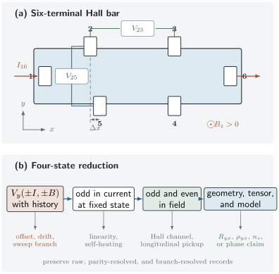
Top: a six-terminal Hall bar with current $I_{16}$, longitudinal voltage $V_{23}$, transverse voltage $V_{25}$, and $B_z$ out of the page. A longitudinal offset $\Delta x$ between transverse contacts mixes part of $V_x$ into $V_y$. Bottom: current reversal, field parity, and geometry or model inference are separate reduction stages; magnetic branches must remain history labeled.

For a homogeneous three-dimensional bar of thickness $t$ with uniform current density,

$$\rho_{yx} = t\,R_{yx}, \qquad \rho_{xx} = R_{xx}\frac{wt}{L}.$$

The Hall conversion does not contain the channel width because the wider current cross section and the longer transverse voltage path cancel in the ideal continuum geometry. That cancellation is not universal for finite voltage arms, invasive metal overlaps, irregular shapes, current jets, edge-dominated transport, or spatially varying conductivity.

For a two-dimensional conducting sheet, $R_{yx}$ is already the sheet Hall resistivity. Converting it to a three-dimensional $\rho_{yx}$ by multiplying by the physical thickness asserts that the current is uniformly distributed through that thickness. Surface states, parallel layers, accumulation regions, and partially depleted films violate that assertion.

Hall-bar design checks

• Current contacts should inject across the channel width without forcing a narrow jet through the voltage region.
• Transverse probes should be narrow and opposed. Wide or overlapping metal probes can shunt the Hall field and distort current flow.
• Longitudinal arms should be separated enough to define $L$ without sitting inside the current-contact spreading region.
• The bar axis and crystallographic axes should be recorded separately.
• Every contact should be tested for linearity, stability, leakage, and acceptable resistance over temperature and field.
• Optical or electron microscopy should document $\Delta x$, channel width, voltage-arm dimensions, cracks, and unintended bridges.

A beautiful lithographic outline does not prove uniform conduction. Spatial variations in carrier density can even produce an incorrect apparent carrier sign in a nominal van der Pauw measurement.

van der Pauw geometry

A uniform, isotropic, simply connected sheet with four sufficiently small contacts on its boundary supports both sheet-resistance and Hall measurements. Current is driven through one opposing contact pair and transverse voltage read across the other; current and field are reversed, and the diagonal configurations are exchanged.

The redundant configurations test contact placement, sample uniformity, reversal consistency, and reciprocity. The method loses its guarantee when contacts lie in the interior, the sample contains a hole, thickness or carrier density varies appreciably, or anisotropy is ignored. Transport Measurements gives the sheet-resistance equation and its geometric assumptions.

From Raw Voltage to Hall Resistance

A useful contamination model

A transverse record can be organized schematically as

$$\begin{aligned} V_y^{\mathrm{raw}} ={}& V_{\mathrm{off}} + I R_{yx}(B,\mathcal H) \\ &+ \epsilon I R_{xx}(B,\mathcal H) + V_{\mathrm{ind}}(\dot B) + V_{\mathrm{th}}. \end{aligned}$$

$\epsilon$ parameterizes longitudinal pickup, often from contact misalignment or current distortion. $V_{\mathrm{off}}$ and $V_{\mathrm{th}}$ need not be field independent, while $V_{\mathrm{ind}}$ depends on sweep rate and loop area. This equation is a diagnostic ledger, not a claim that every artifact adds linearly under all conditions.

Current reversal first

At fixed field and magnetic state, form the current-odd voltage

$$\begin{aligned} V_y^{I-}(B;\mathcal H) ={}& \frac{1}{2} \bigl[ V_y(+I,B;\mathcal H) \\ &\qquad -V_y(-I,B;\mathcal H) \bigr]. \end{aligned}$$

This rejects static current-even offsets. It does not reject Joule-heating contributions that change resistance by an amount proportional to $I^2$ and therefore generate an odd $I^3$ voltage. Several excitation amplitudes are needed to establish a linear range.

Then separate field parity

Write $V^{s_I,s_B}=V_y(s_I I,s_B B)$ for states prepared by a matched protocol. The current-odd, field-odd Hall channel is

$$\begin{aligned} R_{yx}^{I-,B-}(B) ={}& \frac{1}{4I} \bigl[ V^{+,+}-V^{-,+} \\ &\qquad -V^{+,-}+V^{-,-} \bigr]. \end{aligned}$$

The corresponding current-odd, field-even diagnostic is

$$\begin{aligned} R_{yx}^{I-,B+}(B) ={}& \frac{1}{4I} \bigl[ V^{+,+}-V^{-,+} \\ &\qquad +V^{+,-}-V^{-,-} \bigr]. \end{aligned}$$

For a reversible nonmagnetic sample, longitudinal pickup is commonly field even and appears in $R_{yx}^{I-,B+}$, while the ordinary Hall signal appears in $R_{yx}^{I-,B-}$. The decomposition itself is exact for the four numbers. Interpreting the channels requires the two field states to be time-reversed counterparts at the same temperature and configuration.

Reciprocity and lead exchange

Linear-response reciprocity compares a resistance with exchanged current and voltage terminals under reversal of all time-reversal-odd variables. It is a stronger check than field antisymmetrization alone because it changes the lead geometry. Failure can indicate:

• nonlinearity or excessive excitation;
• contact or wiring instability;
• temperature drift;
• magnetic states that were not reversed;
• a genuinely nonreciprocal response outside the assumed regime.

Lead exchange should be planned into the acquisition sequence. Performing it only after an anomalous result is found risks comparing different thermal cycles or aged contacts.

Carrier Density, Sign, and Mobility

One-carrier sheet inference

Define the low-field sheet Hall slope

$$S_{\mathrm H}^{2\mathrm D} \equiv \left. \frac{dR_{yx}^{I-,B-}}{dB} \right|_{B\to0}.$$

For one isotropic carrier type with Hall factor unity,

$$n_s = \frac{1}{e\lvert S_{\mathrm H}^{2\mathrm D}\rvert}, \qquad \operatorname{sgn}(q) = \operatorname{sgn}(S_{\mathrm H}^{2\mathrm D}).$$

Here $e>0$ and $n_s$ is a positive sheet density. A conducting thickness $t$ gives $n=n_s/t$ only if the current-carrying layer is known and uniform.

If the same channel also produces sheet resistance $R_{\square}$, the one-carrier Hall mobility is

$$\mu_{\mathrm H} = \frac{ \lvert S_{\mathrm H}^{2\mathrm D}\rvert }{R_{\square}} = \frac{1}{e n_s R_{\square}}.$$

This is a model-derived mobility, not a directly recorded velocity. Parallel channels, anisotropic scattering, magnetic response, or an energy-dependent relaxation time break the simple identification.

Hall factor

In semiconductor transport, a Hall factor $r_{\mathrm H}$ is often introduced so that the measured slope is $r_{\mathrm H}/(n_s q)$. Then the apparent Hall density is $n_s/r_{\mathrm H}$ and $\mu_{\mathrm H}=r_{\mathrm H}\mu_{\mathrm{drift}}$. The factor depends on band structure, scattering, degeneracy, and temperature. Setting it to one should be stated as an approximation.

Sign discipline

A carrier-sign claim requires:

1. calibrated field polarity at the sample;
2. declared current direction and conventional-current convention;
3. declared transverse voltage polarity;
4. a slope statistically distinguishable from zero;
5. evidence that one-carrier inference is appropriate.

The last condition matters. A positive weak-field slope can coexist with electron pockets if higher-mobility holes dominate the mobility-weighted transverse response. It does not prove that every mobile excitation carries positive charge.

Ordinary, Anomalous, and Quantum Hall Signals

Ordinary Hall response

The simplest ordinary signal is odd in $B$, linear over a stated weak-field interval, nonhysteretic, and consistent across current amplitudes and lead configurations. Its slope may support a one-carrier density when:

• $R_{yx}(B)$ is linear over the relevant range;
• magnetoresistance is modest or understood;
• one band or one carrier type dominates;
• the Hall factor is controlled;
• parallel conduction is negligible;
• geometry and thickness are known.

Linearity alone is insufficient: a multiband conductor can look linear over too narrow a field window, and an anomalous contribution can look linear before magnetization saturates.

Anomalous Hall response

In a magnetic conductor, analysts often write the measured Hall resistivity as an ordinary background plus an anomalous term. Treat this as a model decomposition. Subtracting a high-field line assumes that the ordinary coefficient is field independent and that the anomalous response has reached a known high-field behavior.

A persuasive anomalous-Hall dataset includes:

• magnetic-state preparation and both sweep directions;
• longitudinal and transverse data acquired together;
• magnetization or another order-sensitive measurement under comparable conditions;
• temperature, angle, thickness, and disorder trends;
• tensor conversion rather than a small-Hall-angle shortcut when the angle is not small;
• comparison with symmetry and microscopic calculations.

An anomalous Hall loop need not be proportional to net magnetization. Berry curvature, skew scattering, side jump, noncollinear order, and multiple magnetic regions can contribute. Hall Effect develops those mechanisms.

Quantum Hall response

A quantum Hall claim is based on a correlated longitudinal and transverse pattern, not a flat-looking segment:

• $R_{yx}$ approaches $h/(\nu e^2)$ for an identified integer or fractional $\nu$;
• $R_{xx}$ develops a corresponding minimum and ideally becomes unresolved;
• the feature persists over a field or density interval;
• current is below the breakdown threshold;
• contact and lead mixing are tested;
• temperature and device-size dependence are consistent with the proposed gap and edge transport.

A useful residual is

$$\delta_\nu \equiv \frac{R_{yx}}{h/(\nu e^2)} -1.$$

A small $\delta_\nu$ with appreciable $R_{xx}$ is not yet a metrological plateau. The finite longitudinal signal can mix into $R_{yx}$ and indicates dissipation or incomplete quantization. Integer Quantum Hall Effect gives the canonical phase and edge-state account.

Multiband and Parallel Conduction

Conductivity channels add before the tensor is inverted:

$$\begin{aligned} \boldsymbol{\sigma}_{\mathrm{tot}}(B) &= \sum_a \boldsymbol{\sigma}^{(a)}(B) + \boldsymbol{\sigma}_{\mathrm{parallel}}(B), \\ \boldsymbol{\rho}(B) &= \boldsymbol{\sigma}_{\mathrm{tot}}^{-1}(B). \end{aligned}$$

Consequences include:

• weak-field Hall response weights carrier mobilities more strongly than longitudinal conductivity;
• the sign can differ from the sign of the most numerous carrier type;
• nonlinear $R_{yx}(B)$ can accompany large magnetoresistance;
• a substrate, surface accumulation layer, interface, edge, or damaged region can act as a parallel channel;
• several parameter sets can fit the same finite-field curves.

The familiar two-carrier model contains four positive parameters, $n,p,\mu_e,\mu_h$, before offsets, geometry uncertainty, or field dependence are added. A fit to one Hall curve is therefore weakly identifiable. At minimum:

1. fit $\rho_{xx}(B)$ and $\rho_{yx}(B)$ simultaneously in tensor form;
2. report parameter covariance and sensitivity to the field window;
3. repeat across temperature or gate voltage with physically justified shared parameters;
4. constrain density or Fermi-surface area with capacitance, stoichiometry, spectroscopy, or quantum oscillations;
5. test whether an additional parallel channel changes the conclusion.

Adding a third carrier because residuals remain does not automatically improve physical inference. It may only make a flexible inverse problem less identifiable.

Hysteresis and Magnetic Effects

History is an experimental coordinate

In a magnetic sample, write $R_{yx}(B;\mathcal H)$, not just $R_{yx}(B)$. Relevant histories include:

• upsweep and downsweep;
• positive and negative saturation;
• zero-field cooling and field cooling;
• maximum field reached;
• wait time after a field step;
• temperature and gate trajectory;
• current pulses that can move domains or textures.

Do not antisymmetrize an upsweep at $+B$ with a downsweep at $-B$ unless those points represent the intended time-reversed states. Preserve each branch first. Construct odd and even combinations within explicitly matched preparations, and compare with the Onsager–Casimir relation including magnetization reversal.

Longitudinal and planar Hall mixing

Anisotropic magnetoresistance can generate a planar Hall voltage when magnetization lies in the plane. Its field parity and angular dependence differ from an axial ordinary Hall signal, but domain reversal and misalignment can mix channels. A three-axis angle study should report the actual field vector and mechanical zero, not only the rotator readout.

Residual humps are not direct topology measurements

A common procedure fits an ordinary background, subtracts an anomalous term proportional to magnetization, and labels the remaining hump “topological Hall.” The residual inherits every error in both backgrounds. Multiple magnetic regions with different coercivities or opposite anomalous-Hall signs can create a similar feature without a skyrmion phase.

A real-space-topology claim needs orthogonal evidence such as imaging or scattering, a texture model, field-angle and thickness systematics, and agreement among magnetization, transport, and phase boundaries. Skyrmions and Magnetic Textures owns the real-space topology and emergent-electrodynamics criteria.

Acquisition and Reporting Workflow

1. Map the wiring. Record terminal numbers, lead polarity, channel assignments, current direction, and field-axis calibration.
2. Characterize contacts at zero field. Test linearity, leakage, stability, reciprocity, and current dependence.
3. Choose an excitation range. Demonstrate current-independent $R_{xx}$ and $R_{yx}$; monitor self-heating and phase.
4. Acquire signed states. Measure $\pm I$ at both $\pm B$, exchange lead configurations, and preserve time stamps and zero-current readings.
5. Control field history. Repeat both sweep directions and several rates; perform stabilized field steps at representative points.
6. Reduce without erasing diagnostics. Store raw, current-odd, field-odd, field-even, and branch-resolved channels.
7. Apply geometry and tensor operations. State sheet versus bulk quantities, thickness, sign convention, and whether full inversion was used.
8. Fit the least complex adequate model. Declare field windows, fixed parameters, covariance, residuals, and competing explanations.
9. Cross-check the inference. Compare density, magnetism, or quantization with an independent probe.

A publication-quality dataset should include representative raw sign states, not only the antisymmetrized result. It should also state magnet polarity, sweep rate, current or voltage amplitude, frequency, lock-in phase, filter settings, sample temperature, geometry uncertainty, and every subtraction used.

Uncertainty and Detection Limits

For a one-carrier sheet density $n_s=1/(e|S_{\mathrm H}^{2\mathrm D}|)$, the relative standard uncertainty is approximately

$$\frac{u(n_s)}{n_s} \simeq \frac{ u(S_{\mathrm H}^{2\mathrm D}) }{ \lvert S_{\mathrm H}^{2\mathrm D}\rvert },$$

because $e$ is exact in the SI. The slope uncertainty must include voltage noise, current calibration, field calibration, drift, field-window choice, and correlated residuals. For bulk density $n=n_s/t$, thickness uncertainty and uncertainty in the electrically active layer must be added.

When a symmetric two-field estimate is appropriate,

$$S_{\mathrm H}^{2\mathrm D} \simeq \frac{ V_y^{I-}(+B)-V_y^{I-}(-B) }{ 2IB }.$$

This estimator assumes linearity between the two fields. A regression over many points should report the model, weighting, covariance, and sensitivity to the fit interval. If the inferred slope is comparable to its uncertainty or to uncontrolled longitudinal leakage, the carrier sign is unresolved rather than “small but positive.”

For $\mu_{\mathrm H}=|S_{\mathrm H}^{2\mathrm D}|/R_{\square}$, slope and sheet-resistance uncertainties can be correlated because the same contacts, geometry, temperature, and conduction channels enter both. Propagating them as independent can misstate the mobility uncertainty.

Common Mistakes

• Reporting a carrier sign without a complete voltage, current, field, and tensor convention.
• Antisymmetrizing one current polarity and leaving thermoelectric offsets untested.
• Treating the field-even transverse channel as disposable instead of using it to diagnose longitudinal pickup.
• Pairing different hysteresis branches as though they were time-reversed states.
• Converting a sheet Hall slope to bulk density with the physical rather than electrically active thickness.
• Applying $n_s=1/(e|S_{\mathrm H}|)$ to nonlinear multiband data without a validated one-carrier interval.
• Inferring all Fermi-surface pocket signs from the sign of a mobility-weighted Hall slope.
• Fitting $\rho_{yx}$ with a conductivity expression or inverting tensor elements separately.
• Calling a hysteretic loop proof of one anomalous-Hall mechanism.
• Calling a background-subtracted hump proof of a skyrmion or topological Hall phase.
• Claiming a quantum Hall plateau without simultaneous $R_{xx}$, excitation, temperature, and contact checks.
• Publishing only a symmetrized curve and making the raw sign states unavailable.

Exercises

1. Signed sheet density

With the conventions of this page, a device carrying $I=10.0\,\mu\mathrm A$ at $B=+1.00\,\mathrm T$ has current-odd transverse voltage $V_y^{I-}=-2.00\,\mathrm{mV}$ after field-even pickup is removed. Assume one-carrier linear response. Find the sheet Hall slope, carrier sign, and sheet density.

Solution

The Hall resistance at this field is

$$R_{yx} = \frac{-2.00\,\mathrm{mV}} {10.0\,\mu\mathrm A} = -200\,\Omega.$$

Linearity through the origin gives $S_{\mathrm H}^{2\mathrm D}=-200\,\Omega\,\mathrm T^{-1}$. The negative sign identifies electrons under the declared convention. The sheet density is

$$\begin{aligned} n_s &= \frac{1}{ e\lvert S_{\mathrm H}^{2\mathrm D}\rvert } \\ &= 3.12\times10^{16}\,\mathrm m^{-2} \\ &= 3.12\times10^{12}\,\mathrm{cm}^{-2}. \end{aligned}$$

The result is model conditional: it assumes one carrier type and Hall factor unity.

2. Four-state extraction

At one field magnitude and $I=100\,\mu\mathrm A$, the transverse voltages in microvolts are

$$\begin{aligned} V^{+,+}&=310, & V^{-,+}&=-250, \\ V^{+,-}&=150, & V^{-,-}&=-90. \end{aligned}$$

Find the current-odd response at each field, then the field-odd and field-even transfer resistances.

Solution

At positive and negative field,

$$\begin{aligned} V_y^{I-}(+B) &= \frac{310-(-250)}{2}\,\mu\mathrm V \\ &= 280\,\mu\mathrm V, \\ V_y^{I-}(-B) &= \frac{150-(-90)}{2}\,\mu\mathrm V \\ &= 120\,\mu\mathrm V. \end{aligned}$$

The odd and even voltages are therefore $80\,\mu\mathrm V$ and $200\,\mu\mathrm V$. Dividing by current gives

$$R_{yx}^{I-,B-} = 0.80\,\Omega, \qquad R_{yx}^{I-,B+} = 2.00\,\Omega.$$

The larger field-even channel is consistent with substantial longitudinal pickup. It should be reported and investigated, not silently discarded.

3. Sheet and bulk density

A one-carrier Hall bar has $|S_{\mathrm H}^{2\mathrm D}|=50.0\,\Omega\,\mathrm T^{-1}$. Find $n_s$. If the electrically active thickness is $20.0\,\mathrm{nm}$, find the bulk density. Which result is affected by a ten-percent thickness uncertainty?

Solution

The sheet density is

$$\begin{aligned} n_s &= \frac{1}{e(50.0\,\Omega\,\mathrm T^{-1})} \\ &= 1.25\times10^{17}\,\mathrm m^{-2} \\ &= 1.25\times10^{13}\,\mathrm{cm}^{-2}. \end{aligned}$$

Using $t=20.0\,\mathrm{nm}$,

$$\begin{aligned} n &= \frac{n_s}{t} \\ &= 6.24\times10^{24}\,\mathrm m^{-3} \\ &= 6.24\times10^{18}\,\mathrm{cm}^{-3}. \end{aligned}$$

The sheet density does not require thickness. The bulk density inherits the ten-percent thickness uncertainty, in addition to the Hall-slope uncertainty and the model uncertainty about whether the whole thickness conducts.

4. A positive slope with more electrons

In the weak-field two-carrier model, the Hall numerator is proportional to $p\mu_h^2-n\mu_e^2$. Consider $n=4$ and $p=2$ in common density units, with $\mu_e=1000$ and $\mu_h=2000$ in common mobility units. Determine the Hall sign and explain the lesson.

Solution

The two weighted terms are

$$p\mu_h^2 = 2(2000)^2 = 8.0\times10^6,$$

and

$$n\mu_e^2 = 4(1000)^2 = 4.0\times10^6.$$

The numerator is positive, so the weak-field Hall slope is hole-like even though electrons are twice as numerous. Hall sign is mobility weighted in a multiband conductor; it is not a census of every carrier or Fermi-surface pocket.

5. Hysteresis and antisymmetrization

An analyst combines the $+B$ point from an upsweep after negative saturation with the $-B$ point from a downsweep after positive saturation. The sample is ferromagnetic and both points lie inside its coercive region. Why can the resulting odd component be misleading, and what should be done?

Solution

Inside the coercive region, field does not uniquely determine magnetization or domain state. The two points can represent different mixtures of domains rather than time-reversed versions of one state. Their half-difference mixes Hall parity with branch history.

Keep upsweep and downsweep data separate. Record the saturation protocol and compare points prepared in explicitly related magnetic states. Test reciprocal lead configurations with reversal of both external field and internal magnetic order where possible, and compare with magnetization or imaging under matched conditions.

6. Is this a quantum Hall plateau?

Near a proposed $\nu=2$ plateau, a device gives $R_{yx}=12.910\,\mathrm{k}\Omega$ and $R_{xx}=20\,\Omega$. Use $h/e^2=25\,812.807\,\Omega$ to calculate $\delta_2$. Does the measurement establish a metrological plateau?

Solution

The ideal value is

$$\frac{h}{2e^2} = 12\,906.404\,\Omega.$$

Therefore

$$\begin{aligned} \delta_2 &= \frac{12\,910}{12\,906.404}-1 \\ &= 2.79\times10^{-4}. \end{aligned}$$

The Hall value is close at the $10^{-4}$ level, but $R_{xx}=20\,\Omega$ is clearly nonzero and can mix into the transverse channel. The observation is consistent with an emerging plateau, not by itself with metrological quantization. Current dependence, contact configuration, temperature, field width, and uncertainty must also be checked.

Research Status

• Established: Hall-bar and van der Pauw methods under stated geometry assumptions; current and field reversal; one-carrier sheet-density and Hall-mobility formulas; tensor inversion; Onsager–Casimir reciprocity; integer quantum Hall resistance standards.
• Model dependent: Hall factors, multiband densities and mobilities, electrically active thickness, ordinary-background subtraction, and anomalous-Hall mechanism separation.
• Active: Hall response in noncollinear antiferromagnets, moiré systems, hydrodynamic conductors, nonlinear and nonreciprocal regimes, spatially inhomogeneous devices, and mixed surface–bulk transport.
• Not established by a Hall trace alone: a unique Fermi-surface inventory, one anomalous-Hall mechanism, a skyrmion phase, or topological protection.

Connections

• Transport Measurements supplies the shared four-terminal, current-reversal, sweep, contact, geometry, and uncertainty framework.
• Quantum Oscillations develops orbit-frequency, cyclotron-mass, lifetime, angular, reconstruction, and phase inference from longitudinal, transverse, and thermodynamic field oscillations.
• Hall Effect develops ordinary, multiband, anomalous, Berry-curvature, and quantized Hall theory with a fixed tensor convention.
• Vortex Matter, Pinning, and Flux Flow owns the force, velocity, electric-field, and Hall ledgers for moving superconducting vortices; this page retains transverse-voltage reduction, reversal, admixture, contact, and geometry controls.
• Drude Theory gives the one-carrier Hall benchmark and low-field mobility scale.
• Boltzmann Transport explains mobility weighting, anisotropic bands, and finite-field velocity histories.
• Integer Quantum Hall Effect owns plateau formation, mobility gaps, edge channels, and metrological resistance.
• Conductance Quantization develops coherent terminal response and contact effects.
• Weak Localization shows why longitudinal magnetoconductance must be measured alongside transverse response.
• Skyrmions and Magnetic Textures develops real-space topology and the evidence needed beyond a residual Hall hump.
• Error Estimates provides general tools for regression, conditioning, covariance, and model discrepancy.

Further Reading

• The NIST Hall-measurement archive gives a concrete van der Pauw sequence, sign definitions, redundant configurations, heating limits, and consistency checks.
• D. K. Schroder and R. S. Popović provide broader treatments of semiconductor Hall metrology, contacts, Hall factors, and device geometry.
• N. Nagaosa et al. review ordinary and anomalous mechanisms; read the scaling classifications together with later work that separates residual and phonon scattering.
• M. Büttiker and the integer quantum Hall literature are essential when voltage contacts, edge channels, and coherent terminal boundary conditions replace a local Hall field picture.

References

1. E. H. Hall, “On a New Action of the Magnet on Electric Currents”, American Journal of Mathematics 2, 287–292 (1879).
2. L. J. van der Pauw, “A Method of Measuring Specific Resistivity and Hall Effect of Discs of Arbitrary Shape,” Philips Research Reports 13, 1–9 (1958).
3. National Institute of Standards and Technology, “Resistivity and Hall Measurements”, archived measurement procedure and consistency checks.
4. L. Onsager, “Reciprocal Relations in Irreversible Processes. II”, Physical Review 38, 2265–2279 (1931).
5. H. B. G. Casimir, “On Onsager’s Principle of Microscopic Reversibility”, Reviews of Modern Physics 17, 343–350 (1945).
6. M. Büttiker, “Four-Terminal Phase-Coherent Conductance”, Physical Review Letters 57, 1761–1764 (1986).
7. N. Nagaosa, J. Sinova, S. Onoda, A. H. MacDonald, and N. P. Ong, “Anomalous Hall Effect”, Reviews of Modern Physics 82, 1539–1592 (2010).
8. Y. Tian, L. Ye, and X. Jin, “Proper Scaling of the Anomalous Hall Effect”, Physical Review Letters 103, 087206 (2009).
9. A. Gerber, “Interpretation of Experimental Evidence of the Topological Hall Effect”, Physical Review B 98, 214440 (2018).
10. K. von Klitzing, G. Dorda, and M. Pepper, “New Method for High-Accuracy Determination of the Fine-Structure Constant Based on Quantized Hall Resistance”, Physical Review Letters 45, 494–497 (1980).
11. O. Bierwagen, T. Ive, C. G. Van de Walle, and J. S. Speck, “Causes of Incorrect Carrier-Type Identification in van der Pauw–Hall Measurements”, Applied Physics Letters 93, 242108 (2008).
12. J. G. Gluschke, J. Seidl, H. H. Tan, C. Jagadish, P. Caroff, and A. P. Micolich, “Impact of Invasive Metal Probes on Hall Measurements in Semiconductor Nanostructures”, Nanoscale 12, 20317–20325 (2020).
13. D. K. Schroder, Semiconductor Material and Device Characterization, 3rd ed., Wiley (2006).
14. R. S. Popović, Hall Effect Devices, 2nd ed., Institute of Physics Publishing (2004).
15. C. L. Chien and C. R. West, eds., The Hall Effect and Its Applications, Plenum Press (1980).
16. Joint Committee for Guides in Metrology, Evaluation of Measurement Data—Guide to the Expression of Uncertainty in Measurement, JCGM 100:2008.

Summary

• A Hall measurement begins with signed terminal voltages and a documented magnetic history, not with a carrier density.
• Hall-bar and van der Pauw conversions require uniform current flow, controlled contacts, and a clear sheet-versus-bulk convention.
• Current reversal removes static current-even offsets; field parity separates algebraic channels; reciprocity and branch-resolved protocols test the physical assumptions.
• Carrier sign, density, and mobility follow directly only in a validated one-carrier regime with a controlled Hall factor and electrical thickness.
• Multiband, parallel, anomalous, and magnetic responses require simultaneous longitudinal data and external constraints.
• Quantum or topological claims demand correlated signatures and orthogonal evidence; a plateau-like segment or residual hump is not enough.