Heat Capacity and Thermodynamics

Heat capacity measures how much energy a sample absorbs when its temperature changes under declared constraints. In quantum matter, its low-temperature dependence counts low-energy degrees of freedom without requiring them to carry charge or couple strongly to light. A linear term can constrain a Fermi-surface density of states, a cubic term can reveal acoustic phonons, a sharp anomaly can establish a bulk transition, and an integral of $C/T$ can track entropy released across a broad temperature range.

Calorimetry is bulk-sensitive, but it is not interpretation-free. The thermometer records a platform temperature after heat has flowed through grease, wires, substrate, sample, and bath. The inferred heat capacity includes addenda, can miss a thermally decoupled fraction, and combines electronic, lattice, magnetic, nuclear, defect, and transition contributions. Separating those terms is a model-selection problem, not a subtraction ritual.

A useful evidence ladder is:

1. thermal record: heater power and thermometer resistance or temperature versus time, frequency, or scan coordinate;
2. calorimeter response: total platform-plus-sample heat capacity and thermal conductance under a validated heat-flow model;
3. sample heat capacity: addenda-subtracted $C_p$, $C_V$, or an effective dynamic heat capacity with units, amount convention, field, pressure, and protocol stated;
4. component inference: electronic, phonon, magnetic, nuclear, defect, or transition contribution after a constrained background analysis;
5. material claim: density of states, gap structure, bulk phase transition, entropy release, phase fraction, or critical behavior supported by complementary probes and uncertainty propagation.

A peak is a thermodynamic anomaly. Its microscopic identity and transition order require more evidence than its position.

Canonical Scope

This page is the canonical home for heat-capacity measurement and thermodynamic inference in quantum materials. It owns relaxation, heat-pulse, and ac calorimetry; addenda and thermal-link models; the distinction among total, specific, molar, and volumetric heat capacities; low-temperature component separation; entropy integration; bulk transition diagnostics; and the experimental cautions behind electronic, phonon, superconducting, magnetic, Schottky, and quantum-critical interpretations.

Thermodynamic Potentials owns Legendre transforms and natural variables. Entropy owns statistical definitions and thermodynamic identities. Sommerfeld Expansion derives the ideal degenerate-fermion heat capacity and fixed-number correction. Phonons derives harmonic lattice heat capacity, the Debye law, mode Grüneisen parameters, and thermal expansion. Finite-Temperature Phase Transitions owns transition order, latent heat, critical exponents, and finite-size scaling.

BCS Theory owns the superconducting entropy and weak-coupling heat-capacity benchmark. Heavy Fermions and Quantum Criticality own material-specific coherence and critical-scaling claims. The present page explains how calorimetry constrains those theories and where that inference can fail.

Heat-Capacity Conventions

State the held variables

For a reversible path with generalized controls $X$ held fixed,

$$C_X = T \left( \frac{\partial S}{\partial T} \right)_X = \left( \frac{\delta Q_{\mathrm{rev}}}{dT} \right)_X.$$

At constant volume,

$$C_V = \left( \frac{\partial U}{\partial T} \right)_{V,N,\ldots},$$

whereas at constant pressure,

$$C_p = \left( \frac{\partial H}{\partial T} \right)_{p,N,\ldots}.$$

Low-pressure calorimetry on a freely expanding solid usually approximates $C_p$. Many microscopic models calculate $C_V$. For an isotropic equilibrium solid,

$$C_p-C_V = \frac{ TV\alpha_V^2 }{ \kappa_T } = TVB_T\alpha_V^2,$$

where $\alpha_V$ is the volume expansion coefficient, $\kappa_T$ the isothermal compressibility, and $B_T=1/\kappa_T$. The difference is often small at cryogenic temperatures, but it can matter near structural transitions, soft modes, and large thermal expansion.

Magnetic field, pressure, strain, composition, and particle number also belong to the constraint ledger. A field-swept or pressure-swept calorimetric protocol is not automatically the same derivative as a temperature sweep at fixed field or pressure.

Extensive and normalized quantities

Use distinct notation and units for:

• total heat capacity $C$ in $\mathrm{J\,K^{-1}}$;
• mass-specific heat capacity $c=C/m$ in $\mathrm{J\,kg^{-1}\,K^{-1}}$;
• molar heat capacity $C_m=C/n_{\mathrm{mol}}$ in $\mathrm{J\,mol^{-1}\,K^{-1}}$;
• volumetric heat capacity $C/V$ in $\mathrm{J\,m^{-3}\,K^{-1}}$.

In materials papers, “specific heat” often means molar heat capacity. That usage is conventional but ambiguous. State whether one mole means formula units, atoms, magnetic ions, or another counted object. The distinction enters every comparison with $R\ln g$, $3nR$, a Sommerfeld coefficient, or a phase fraction.

What a Calorimeter Measures

Relaxation calorimetry

A common low-temperature calorimeter mounts a sample on a small platform containing a heater and thermometer. A weak thermal link of conductance $K$ connects the platform to a bath at temperature $T_b$. In the one-node, small-excursion model,

$$C_{\mathrm{tot}} \frac{d\delta T}{dt} = P(t)-K\delta T, \qquad \delta T = T-T_b.$$

After the heater is switched off,

$$\delta T(t) = \delta T_0e^{-t/\tau}, \qquad \tau = \frac{C_{\mathrm{tot}}}{K}.$$

The sample heat capacity is then inferred from

$$C_{\mathrm{samp}} = C_{\mathrm{tot}} -C_{\mathrm{add}},$$

where $C_{\mathrm{add}}$ includes the platform, thermometer, heater, leads, grease, and any substrate or capsule that participates thermally.

This simple exponential is valid only when the sample and platform share one temperature, $C$ and $K$ are effectively constant across the pulse, the bath remains fixed, radiative and parasitic heating are negligible, and the transition does not release latent heat during the decay. A good fit residual is necessary but not sufficient: several thermal modes can masquerade as one over a short time window.

Internal thermalization and the two-node model

Poor sample contact or low internal thermal diffusivity creates a second time scale. A minimal two-node model uses a sample temperature $T_s$, platform temperature $T_a$, sample–platform conductance $K_s$, and bath conductance $K_b$:

$$\begin{aligned} C_s\dot T_s &= -K_s(T_s-T_a), \\ C_a\dot T_a &= P(t) -K_b(T_a-T_b) +K_s(T_s-T_a). \end{aligned}$$

The platform response is generally a sum of two exponentials. The fast internal mode tests whether the sample equilibrates with the thermometer; the slow external mode describes cooling to the bath. If the time scales are not resolved or the sample has distributed thermal diffusion, a lumped two-node fit can still bias $C_s$.

Thermal grease improves contact but adds heat capacity. A tiny crystal with heat capacity much smaller than the addenda is obtained as a difference between comparable numbers, amplifying mass, fit, and background uncertainty. Measuring the empty platform under the same field, temperature, wiring, and grease protocol is essential.

Heat-pulse and ac methods

In a nearly adiabatic heat-pulse measurement,

$$Q = \int P(t)\,dt \simeq \int_{T_i}^{T_f} C(T)\,dT.$$

Small pulses give $C\simeq Q/\Delta T$; larger pulses average across the interval and can resolve or obscure a transition depending on the analysis. A first-order transition is often better handled by energy accounting than by forcing a relaxation time through a latent-heat plateau.

In ac calorimetry, sinusoidal power $P_\omega$ produces a temperature oscillation. For one thermal node,

$$\lvert T_\omega\rvert = \frac{ \lvert P_\omega\rvert }{ \sqrt{ K^2+(\omega C)^2 } }, \qquad \tan\phi = \frac{\omega C}{K}.$$

In the useful intermediate-frequency window where heat leakage is slow but internal equilibration remains fast,

$$C \simeq \frac{ \lvert P_\omega\rvert }{ \omega\lvert T_\omega\rvert }.$$

Ac calorimetry can have excellent relative sensitivity and reject slow drift, especially for tiny samples or pressure cells. Its absolute scale depends on heater calibration, phase, thermal links, and the frequency window. A frequency-dependent “heat capacity” can itself reveal slow internal degrees of freedom, but it is then a dynamic response rather than an equilibrium $C_p$.

Thermometer and protocol controls

The thermometer must be calibrated in temperature and field on the mounted platform. Self-heating, magnetoresistance, field-sweep eddy currents, wiring heat leaks, bath drift, and finite controller bandwidth can all create false anomalies. The heater power is $P=I^2R$ only after current, heater resistance, waveform, and lead configuration are known at the measurement condition.

Useful controls include:

1. empty-platform and reference-material runs;
2. several pulse sizes or ac frequencies;
3. warming and cooling;
4. repeated points and reordered scans;
5. several sample masses or mountings;
6. magnetic-field and sweep-rate checks;
7. raw relaxation curves and fit residuals near anomalies.

Decomposing the Total Heat Capacity

Write the measured molar heat capacity schematically as

$$C_m = C_{\mathrm{el}} +C_{\mathrm{ph}} +C_{\mathrm{mag}} +C_{\mathrm{nuc}} +C_{\mathrm{def}} +C_{\mathrm{tr}} +\cdots.$$

This decomposition organizes analysis, but it is not exact when sectors are strongly coupled. Magnetoelastic modes, electron–phonon renormalization, hybridization, and collective order can redistribute entropy between nominal components. A background should therefore be described as a model for the non-target terms, not as the uniquely known lattice or electronic heat capacity.

Useful background strategies include:

• a low-temperature expansion over a justified asymptotic window;
• a field-suppressed normal state, if field does not substantially alter other terms;
• an isostructural nonmagnetic analog with mass and phonon corrections;
• a first-principles or measured phonon density of states;
• a global fit constrained simultaneously by several fields, compositions, or pressure values.

Each strategy has failure modes. A nonmagnetic analog can have different force constants or electronic structure. A high field can add Zeeman and nuclear terms. A polynomial can absorb the anomaly being sought.

Electronic Heat Capacity

Sommerfeld coefficient

For a Fermi liquid at temperatures small compared with the relevant Fermi scale,

$$C_{\mathrm{el}} = \gamma T +O(T^3),$$

with

$$\gamma = \frac{\pi^2}{3} k_{\mathrm B}^2 D^*(E_{\mathrm F}).$$

Here $D^*(E_{\mathrm F})$ is the interacting quasiparticle density of states including both spin projections in the same amount convention as $\gamma$. The Sommerfeld Expansion derives the ideal-gas result. In a material, mass renormalization, band multiplicity, electron–phonon coupling, and correlations enter the measured coefficient.

In an ordinary three-dimensional metal whose leading phonon term is $\beta T^3$,

$$\frac{C_m}{T} = \gamma +\beta T^2 +\delta T^4 +\cdots.$$

A $C_m/T$ versus $T^2$ plot makes $\gamma$ the intercept and $\beta$ the initial slope only within the asymptotic regime. Curvature, superconductivity, magnetism, nuclear terms, Schottky tails, dimensional crossover, or a non-Fermi-liquid contribution invalidate a two-parameter straight-line fit.

What a large gamma means

A large $\gamma$ establishes a large low-energy entropy density relative to temperature. In a coherent Fermi liquid it corresponds to a large quasiparticle density of states and often a large effective mass. It does not alone prove a heavy-fermion ground state, identify which bands are heavy, or distinguish intrinsic quasiparticles from low-energy disorder, two-level systems, or unresolved magnetic contributions.

The Wilson ratio combines $\gamma$ with the spin susceptibility and can test a quasiparticle interpretation, but only after core diamagnetism, Van Vleck terms, $g$ factors, and amount conventions are aligned. Quantum oscillations, ARPES, transport, and magnetic response provide independent constraints.

Phonon Heat Capacity

Debye coefficient

For a three-dimensional crystal with gapless acoustic phonons and linear long-wavelength dispersion,

$$C_{\mathrm{ph}} = \beta T^3 +O(T^5).$$

When $C_m$ is per mole of formula units containing $n$ atoms,

$$\beta = \frac{ 12\pi^4 }{ 5 } \frac{ nR }{ \Theta_{\mathrm D}^3 },$$

so an effective low-temperature Debye temperature is

$$\Theta_{\mathrm D} = \left( \frac{ 12\pi^4nR }{ 5\beta } \right)^{1/3}.$$

This $\Theta_{\mathrm D}$ summarizes the acoustic density of states sampled in the fit window. It need not equal a Debye temperature inferred from elastic constants, diffraction, a full-temperature fit, or another convention.

At temperatures above all harmonic phonon scales, the lattice contribution approaches the Dulong–Petit limit $3nR$ per mole of formula units. Real measurements can deviate because optical modes are not yet saturated, thermal expansion converts $C_V$ to $C_p$, anharmonicity changes frequencies, electronic or magnetic terms persist, or a structural transition intervenes.

Beyond one cubic term

The $T^3$ law assumes three-dimensional linear acoustic branches and a sufficiently low temperature. Layered crystals can show crossovers rather than a pure two-dimensional power law because any finite interlayer coupling restores three-dimensional behavior at the longest wavelength. Soft optical modes, rattling modes, disorder, vacancies, and anharmonicity add non-Debye structure.

An Einstein-like optical contribution has the form

$$C_E = N_Ek_{\mathrm B} \left( \frac{\Theta_E}{T} \right)^2 \frac{ e^{\Theta_E/T} }{ \left( e^{\Theta_E/T}-1 \right)^2 },$$

but fitting several Einstein temperatures is descriptive unless spectroscopy or a phonon calculation constrains the modes and weights. A broad phonon density of states should not be turned into a collection of physically named oscillators merely because the fit is excellent.

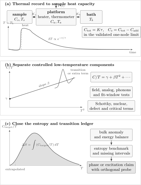
Calorimetric inference has three layers: a heat-flow model converts heater and thermometer records into sample heat capacity; controlled low-temperature fits separate candidate components; and integration of $C/T$ tests entropy balance and bulk transition claims. Addenda, internal relaxation, field-dependent backgrounds, and extrapolation below the base temperature remain part of the result.

Phase Transitions

What an anomaly establishes

Heat capacity is a second temperature derivative of a thermodynamic potential. It is therefore sensitive to bulk nonanalyticity even when a minority conductive path dominates transport or a surface probe sees only a reconstructed layer. Reproducible entropy-carrying anomalies are strong evidence that a finite sample volume participates.

They are not self-labeling. A lambda-shaped peak can arise near a continuous magnetic, structural, charge-order, ferroelectric, or superconducting transition. A broad maximum can be a crossover, short-range order, a Schottky anomaly, a glassy distribution, or a strongly broadened transition. Identify the order parameter with a symmetry-sensitive measurement.

Continuous transitions

Near a continuous transition at $T_c$, define reduced temperature

$$t = \frac{T-T_c}{T_c}.$$

The singular contribution is often parameterized as

$$C_{\mathrm{sing}} = A_\pm \lvert t\rvert^{-\alpha},$$

with different amplitudes above and below $T_c$ plus analytic backgrounds and corrections to scaling. If $\alpha<0$, the heat capacity has a finite cusp rather than a divergence. Thus absence of an infinite peak does not exclude a continuous transition.

Real anomalies are rounded by finite resolution, sample inhomogeneity, strain, disorder, finite size, temperature gradients, and pulse averaging. Fitting a critical exponent requires a reduced-temperature window wide enough to resolve scaling but narrow enough to suppress regular backgrounds and crossover physics. The transition temperature, amplitudes, background, correction terms, and convolution width are correlated; they should not be fixed opportunistically.

First-order transitions and latent heat

At an ideal equilibrium first-order transition, the entropy jumps by $\Delta S$ and the latent heat is

$$L = T_t\Delta S.$$

Formally, a temperature scan contains

$$C_p(T) = C_{\mathrm{reg}}(T) +L\delta(T-T_t).$$

A finite experiment spreads that energy over time and temperature. A relaxation curve may pause, develop multiple slopes, or become history dependent, violating the single-exponential model. The integrated heat, warming–cooling hysteresis, sweep-rate dependence, coexistence, and structural or magnetic state should be examined. Hysteresis alone does not prove equilibrium first order because thermal lag and slow kinetics can also produce it.

Superconducting transitions

For weak-coupling isotropic BCS theory,

$$\frac{ \Delta C_{\mathrm{el}}(T_c) }{ \gamma_nT_c } \simeq 1.426.$$

This is a benchmark, not a universal criterion. Strong coupling, gap anisotropy, multiple bands, pair breaking, fluctuations, transition broadening, and incomplete superconducting volume all change the measured jump. A field-suppressed normal-state reference is useful only if the field does not introduce comparably important magnetic, nuclear, vortex, or normal-state changes.

Thermodynamic consistency requires entropy balance at a continuous zero-field transition:

$$\int_0^{T_c} \frac{ C_s(T)-C_n(T) }{ T } \,dT = 0.$$

Failure can expose an incorrect background, missing low-temperature extrapolation, transition broadening, or a normal-state model that is not physically accessible. A residual linear term $\gamma_0T$ below $T_c$ can come from nodes plus disorder, impurity states, metallic inclusions, nonsuperconducting volume, vortex cores, or an underestimated nuclear subtraction. It is not a unique gap-symmetry diagnostic.

Magnetic and structural transitions

A magnetic heat-capacity anomaly establishes entropy redistribution but not the ordering wavevector or moment direction. Combine it with Neutron Scattering, calibrated magnetic susceptibility, local probes, or diffraction.

Structural transitions can produce large phonon and latent-heat contributions. Electronic order may be coupled strongly enough that “electronic” and “lattice” entropy cannot be separated uniquely. The full anomaly can still establish a bulk transition and constrain the total entropy, while microscopic partitioning remains model dependent.

Entropy Accounting

Integrating measured heat capacity

Along a path with the same fixed controls,

$$S(T_2)-S(T_1) = \int_{T_1}^{T_2} \frac{C_X(T)}{T} \,dT.$$

Calorimetry therefore measures entropy differences, not an absolute zero by itself. To quote $S(T)$ from zero temperature, one must invoke the third law for the relevant equilibrium state and estimate the unmeasured interval below the base temperature.

For a separated magnetic contribution,

$$S_{\mathrm{mag}}(T) = \int_0^T \frac{ C_{\mathrm{mag}}(T') }{ T' } \,dT'.$$

The result inherits every baseline choice. Because division by $T$ emphasizes low-temperature errors, a small residual addenda or nuclear term can create a substantial entropy bias.

Entropy benchmarks

One mole of independent local objects with accessible degeneracy $g$ has an ideal entropy scale

$$S = R\ln g.$$

For a Kramers doublet, this is $R\ln2$. Recovering less entropy by the highest measured temperature does not automatically imply missing degrees of freedom. Entropy may lie above the integration window because of exchange, Kondo screening, crystal-field levels, a broad crossover, or an incorrect background. Recovering more than the expected value usually signals additional levels, phonon mismatch, amount normalization, or subtraction error.

Entropy can be released well above an ordering transition by short-range correlations. The area immediately under a sharp anomaly therefore need not equal the full local-moment entropy. Conversely, a small anomaly can represent a bulk transition from a state whose entropy was already removed gradually.

Free-energy differences

If a reference state and ordered state meet continuously at $T_c$, define

$$\Delta C = C_{\mathrm{ord}}-C_{\mathrm{ref}}, \qquad \Delta S(T) = \int_0^T \frac{\Delta C(T')}{T'} \,dT'.$$

With $\Delta F(T_c)=0$,

$$\Delta F(T) = \int_T^{T_c} \Delta S(T')\,dT'.$$

For a stable ordered state, $\Delta F<0$ below $T_c$. This construction can estimate a superconducting condensation energy or compare competing phases, but only if the extrapolated reference is physically justified and the same amount and field conventions are used.

Low-Temperature Signatures

Gapped and nodal excitations

For a clean fully gapped sector with minimum gap $\Delta$, the low-temperature heat capacity is exponentially suppressed,

$$C_{\mathrm{gap}} \sim T^a e^{-\Delta/(k_{\mathrm B}T)},$$

where the prefactor power $a$ depends on the dispersion and dimensionality. A power law can indicate nodes or gapless collective modes. For example, a quasiparticle density of states proportional to $E$ gives $C\propto T^2$, while point-node-like $D(E)\propto E^2$ gives $C\propto T^3$.

These exponents are not unique labels. Impurity scattering can create residual density of states and crossovers; phonons also contribute $T^3$ in three dimensions; magnons can produce several powers depending on gap, dispersion, and dimensionality. Fit over sliding temperature windows, compare field dependence, and use momentum- or symmetry-sensitive probes.

Schottky anomalies

Independent two-level objects with degeneracies $g_0$ and $g_1$, splitting $\Delta$, and molar fraction $f$ contribute

$$C_{\mathrm{Sch}} = fR x^2 \frac{ g_0g_1e^{-x} }{ \left( g_0+g_1e^{-x} \right)^2 }, \qquad x = \frac{\Delta}{k_{\mathrm B}T}.$$

For equal degeneracies, the maximum occurs near

$$k_{\mathrm B}T_{\max} \simeq 0.417\Delta,$$

and the total entropy approaches $fR\ln2$. Crystal-field levels, paramagnetic impurities, tunneling defects, and nuclear Zeeman or quadrupole levels can all create Schottky-like structure. Tracking the peak with magnetic field and checking its integrated entropy constrain the level scheme.

At temperatures high compared with a small nuclear splitting, a nuclear contribution often has the tail

$$C_{\mathrm{nuc}} \simeq \frac{A(H)}{T^2}.$$

Dividing by $T$ makes this rise as $T^{-3}$ in $C/T$, so it can dominate the apparent low-temperature intercept. The exact coefficient depends on isotope abundance, nuclear spin, hyperfine and quadrupole interactions, and field orientation.

Heavy fermions and quantum criticality

A large, nearly constant $C/T$ at low temperature is a defining thermodynamic signature of a heavy Fermi liquid when accompanied by coherent transport and compatible magnetic or spectroscopic evidence. The crossover into coherence can redistribute entropy over a broad range. Crystal-field and Kondo scales complicate subtraction of a nonmagnetic analog.

Near a quantum critical point, $C/T$ may grow logarithmically or with a fractional power, but no single form is universal. Nuclear terms, disorder, Griffiths-like distributions, dimensional crossover, and a nearby classical transition can imitate or mask a divergence. Quantum Criticality owns the scaling, entropy-ridge, thermal-expansion, and Grüneisen tests needed for a critical claim.

Insulators and amorphous contributions

A clean three-dimensional crystalline insulator should lose its electronic linear term, leaving phonons and any magnetic excitations. A measured $C\propto T$ term in an electrical insulator can arise from tunneling two-level systems in an amorphous fraction, defects, metallic inclusions, spinons, or other gapless excitations. The coefficient alone does not identify a quantum spin liquid.

A broad low-temperature maximum likewise does not establish a phase transition. Search for size or frequency dependence, field evolution, hysteresis, symmetry breaking, and the entropy expected from the proposed degrees of freedom.

A Defensible Workflow

1. Define the derivative and normalization

State $C_p$, $C_V$, or dynamic heat capacity; fixed magnetic field, pressure, and strain; total, molar, mass-specific, or volumetric units; and the object counted by one mole. Record sample mass, composition, formula mass, and uncertainty.

2. Validate the thermal model

Measure addenda, inspect complete heating and cooling curves, compare one- and two-time-constant fits, vary pulse amplitude or ac frequency, and verify sample–platform coupling. Preserve the raw time series near every anomaly.

3. Bound instrumental systematics

Calibrate thermometer and heater in field, test bath stability and sweep-rate dependence, repeat mountings or reference samples, and propagate addenda uncertainty. A sample contribution comparable to or smaller than the addenda requires especially conservative error bars.

4. Separate components globally

Fit a physically justified temperature window and compare several background strategies. Use fields, nonmagnetic analogs, spectroscopic phonons, or normal-state data as constraints rather than independent excuses to subtract. Report parameter covariance and sensitivity to fit window.

5. Integrate an entropy ledger

Show measured, extrapolated, and subtracted intervals separately. State the low-temperature extrapolation, the upper integration limit, and the benchmark entropy. Check entropy balance across continuous transitions and energy balance across first-order ones.

6. Combine orthogonal probes

Use diffraction or scattering for symmetry and wavevector, susceptibility for magnetic response, transport for charge dynamics, and spectroscopy for gaps or modes. Calorimetry establishes bulk entropy; another probe usually identifies which degree of freedom carries it.

Observable Ledger

Reported quantity	Directly constrained by	Main additional assumptions
$C_{\mathrm{tot}}$	Heater and thermometer response	Heat-flow model, $K$, thermometer and heater calibration
$C_{\mathrm{samp}}$	Loaded minus addenda calorimeter	Reproducible mount and participating sample fraction
$\gamma$	Low-$T$ intercept of $C/T$	Valid electronic plus phonon model and bounded extra terms
$\Theta_{\mathrm D}$	Cubic coefficient $\beta$	Three-dimensional acoustic asymptote and atom convention
$\Delta C(T_c)$	Resolved anomaly and normal background	Transition width, phase fraction and reference state
$S_{\mathrm{mag}}$	Integral of background-subtracted $C/T$	Lattice model and low-$T$ extrapolation
Gap structure	Exponential or power-law trend	Purity, field, dimensionality and competing excitations
Transition order	Latent heat, discontinuity and coexistence	Equilibrium protocol, sweep-rate and thermal-lag controls

Common Mistakes

1. Calling every measured quantity specific heat. Total, mass-specific, molar, and volumetric quantities have different units.
2. Comparing $C_p$ data directly with a $C_V$ model without checking expansion. The difference can matter near soft or structural physics.
3. Subtracting addenda measured under another mounting or field condition. Grease, thermometer, and platform contributions change.
4. Accepting a one-exponential fit when the sample is internally slow. Thermally decoupled volume can be missed.
5. Forcing relaxation calorimetry through latent heat. First-order transitions violate the smooth one-node model.
6. Reading $\gamma$ and $\beta$ from any straight-looking $C/T$ plot. The intercept and slope are asymptotic quantities.
7. Treating a fitted Debye temperature as unique. Different observables weight the phonon spectrum differently.
8. Using a nonmagnetic analog as an exact lattice subtraction. Mass, volume, bonding, and force constants can differ.
9. Interpreting a reduced superconducting jump as one mechanism. Gap anisotropy, volume fraction, broadening, and background all matter.
10. Integrating $C/T$ without showing extrapolations. The unmeasured low-temperature interval can control the entropy.
11. Equating $R\ln2$ with proof of localized spin-$1/2$ moments. Other two-level sectors and crystal-field schemes can share that entropy.
12. Calling a broad Schottky or short-range-order maximum a phase transition. A crossover need not break symmetry or carry latent heat.
13. Assigning a power law from less than a decade. Nearby terms can create an effective exponent.
14. Calling a linear term in an insulator a spinon Fermi surface. Defects, glassy two-level systems, and metallic inclusions must be bounded.

Exercises

1. Extract a sample heat capacity

A loaded relaxation calorimeter has slow time constant $\tau=4.80\ \mathrm s$ and bath conductance $K=0.250\ \mathrm{mW\,K^{-1}}$. The measured addenda heat capacity is $0.350\ \mathrm{mJ\,K^{-1}}$. Find the sample heat capacity.

Solution

The total heat capacity is

$$\begin{aligned} C_{\mathrm{tot}} &= K\tau \\ &= (0.250\ \mathrm{mJ\,s^{-1}\,K^{-1}}) (4.80\ \mathrm s) \\ &= 1.20\ \mathrm{mJ\,K^{-1}}. \end{aligned}$$

Therefore

$$C_{\mathrm{samp}} = 1.20-0.350 = 0.850\ \mathrm{mJ\,K^{-1}}.$$

This result assumes the one-node model. A resolved fast internal time or a poor residual would require a two-node or distributed analysis.

2. Infer gamma and a Debye temperature

A five-atom metallic formula unit has a low-temperature fit

$$\frac{C_m}{T} = 25.0 +0.400T^2$$

in $\mathrm{mJ\,mol^{-1}\,K^{-2}}$, with the slope in $\mathrm{mJ\,mol^{-1}\,K^{-4}}$. Find $\gamma$ and the effective $\Theta_{\mathrm D}$.

Solution

The intercept is

$$\gamma = 25.0\ \mathrm{mJ\,mol^{-1}\,K^{-2}}.$$

Using $\beta=0.400\ \mathrm{mJ\,mol^{-1}\,K^{-4}}=4.00\times10^{-4}\ \mathrm{J\,mol^{-1}\,K^{-4}}$ and $n=5$,

$$\begin{aligned} \Theta_{\mathrm D} &= \left( \frac{ 12\pi^4(5)R }{ 5\beta } \right)^{1/3} \\ &\simeq 290\ \mathrm K. \end{aligned}$$

This is the low-temperature acoustic Debye scale for the stated mole convention, not a unique full-spectrum temperature.

3. Compare constant-pressure and constant-volume heat capacities

At $300\ \mathrm K$, a solid has molar volume $V_m=1.00\times10^{-5}\ \mathrm{m^3\,mol^{-1}}$, volume expansion coefficient $\alpha_V=3.00\times10^{-5}\ \mathrm{K^{-1}}$, and isothermal bulk modulus $B_T=100\ \mathrm{GPa}$. Estimate $C_p-C_V$ per mole.

Solution

Using

$$C_p-C_V = TV_mB_T\alpha_V^2,$$

gives

$$\begin{aligned} C_p-C_V &= (300) (1.00\times10^{-5}) (1.00\times10^{11}) (3.00\times10^{-5})^2 \\ &= 0.270\ \mathrm{J\,mol^{-1}\,K^{-1}}. \end{aligned}$$

This is small compared with a Dulong–Petit-scale lattice heat capacity, but it is not identically zero.

4. Audit a magnetic entropy

After background subtraction, a material has

$$\int_0^{2\,\mathrm K} \frac{C_{\mathrm{mag}}}{T}\,dT = 0.20\ \mathrm{J\,mol^{-1}\,K^{-1}},$$

and $C_{\mathrm{mag}}/T=0.50\ \mathrm{J\,mol^{-1}\,K^{-2}}$ from $2$ to $8\ \mathrm K$. What entropy is recovered by $8\ \mathrm K$, and what fraction is this of $R\ln2$?

Solution

The measured contribution from $2$ to $8\ \mathrm K$ is

$$\Delta S = (0.50)(8-2) = 3.00\ \mathrm{J\,mol^{-1}\,K^{-1}}.$$

Including the stated low-temperature interval,

$$S_{\mathrm{mag}}(8\ \mathrm K) = 3.20\ \mathrm{J\,mol^{-1}\,K^{-1}}.$$

Since

$$R\ln2 \simeq 5.76\ \mathrm{J\,mol^{-1}\,K^{-1}},$$

the recovered fraction is about $0.556$. The missing entropy could occur above $8\ \mathrm K$, have been removed by correlations over a wider range, or reflect a background or amount-convention error; the integral alone does not choose among them.

5. Locate a Schottky splitting

An equal-degeneracy two-level Schottky anomaly peaks at $T_{\max}=4.17\ \mathrm K$. Estimate $\Delta/k_{\mathrm B}$. What entropy is recovered at high temperature for one mole of such two-level objects?

Solution

For equal degeneracies,

$$T_{\max} \simeq 0.417 \frac{\Delta}{k_{\mathrm B}},$$

so

$$\frac{\Delta}{k_{\mathrm B}} \simeq \frac{4.17\ \mathrm K}{0.417} = 10.0\ \mathrm K.$$

Once both levels are thermally populated, the entropy approaches

$$S = R\ln2.$$

A smaller integrated entropy would imply a fraction less than one, incomplete temperature coverage, unequal assumptions, or subtraction error.

6. Enforce superconducting entropy balance

Consider a toy normal-state electronic heat capacity $C_n=\gamma T$ and a toy superconducting form $C_s=aT^2$ for $0<T<T_c$. Determine $a$ from entropy balance at $T_c$, then find $\Delta C/(\gamma T_c)$.

Solution

Entropy balance requires

$$\int_0^{T_c} \frac{C_s-C_n}{T} \,dT = 0.$$

Therefore

$$\int_0^{T_c} \left( aT-\gamma \right) \,dT = \frac{aT_c^2}{2} -\gamma T_c = 0,$$

so

$$a = \frac{2\gamma}{T_c}.$$

At the transition,

$$C_s(T_c) = 2\gamma T_c, \qquad C_n(T_c) = \gamma T_c,$$

and hence

$$\frac{\Delta C}{\gamma T_c} = 1.$$

The value differs from the BCS benchmark because the assumed $T^2$ form is only a toy model. The exercise shows that entropy balance constrains the entire curve, not just the jump.

7. Audit a low-temperature linear term

An electrically insulating crystal has $C/T=\gamma_0+\beta T^2$ between $0.35$ and $1.0\ \mathrm K$. A report identifies $\gamma_0$ as a spinon Fermi surface. What tests are needed?

Solution

The linear term establishes low-energy entropy with an approximately linear heat capacity in that window. A spinon interpretation should additionally test:

1. addenda, sample coupling, thermometer self-heating, and fit-window stability;
2. metallic inclusions or surface conduction through composition, microscopy, and transport bounds;
3. amorphous fractions and tunneling two-level systems through sample-quality and preparation dependence;
4. nuclear and paramagnetic Schottky terms through field dependence and lower-temperature data;
5. magnetic entropy over a broad temperature range and the expected moment count;
6. thermal conductivity, magnetic susceptibility, NMR, neutron scattering, or another independent probe of gapless spin excitations;
7. disorder and field scaling against explicit spin-liquid and impurity models;
8. reproducibility across crystals and mountings.

Until those alternatives are bounded, “residual linear heat-capacity term” is the defensible observation.

Research Status

• Established: thermodynamic heat-capacity identities, relaxation and ac heat-flow models, addenda subtraction, Sommerfeld and Debye asymptotes, entropy integration, Schottky response, latent heat, and bulk calorimetric transition signatures.
• Model dependent: decomposition into electronic, lattice, magnetic, and defect sectors; effective Debye temperatures; gap extraction; superconducting volume fractions; nonmagnetic-analog subtraction; and critical exponents from finite windows.
• Active: nanocalorimetry, calorimetry under extreme pressure and field, frequency-dependent heat capacity of slow quantum matter, multimodal calorimetry with scattering, and uncertainty-aware extraction of coupled entropy sectors.
• Unsupported without controls: identifying a novel phase, gap symmetry, spinon Fermi surface, quantum critical point, or microscopic order from one heat-capacity power law or anomaly.

Cross-Links

• Unconventional Superconductivity places entropy-balanced transition anomalies and low-temperature power laws into a multi-probe pairing-symmetry ledger; this page retains calorimeter response, subtraction, normalization, and entropy accounting.
• How Quantum Matter Is Measured gives the general detector-to-claim and uncertainty framework.
• Thermodynamic Potentials fixes natural variables, Legendre transforms, and response derivatives.
• Entropy develops statistical and thermodynamic entropy.
• Sommerfeld Expansion derives the low-temperature ideal-fermion expansion.
• Phonons develops lattice modes, harmonic heat capacity, Debye behavior, and quasiharmonic expansion.
• Finite-Temperature Phase Transitions owns latent heat, coexistence, critical scaling, and transition order.
• BCS Theory derives superconducting entropy, condensation energy, and the weak-coupling jump.
• Heavy Fermions connects large low-temperature entropy to coherent heavy quasiparticles.
• Quantum Criticality develops critical thermodynamics, thermal expansion, and Grüneisen diagnostics.
• Magnetic Susceptibility connects bulk moment records to magnetic response components, ordered-state tests, and field-history controls.
• Neutron Scattering identifies magnetic and lattice modes that calorimetry counts only in aggregate.

References

1. T. H. K. Barron and G. K. White, Heat Capacity and Thermal Expansion at Low Temperatures (Springer, 1999), doi:10.1007/978-1-4615-4695-5.
2. E. S. R. Gopal, Specific Heats at Low Temperatures (Plenum Press, 1966).
3. G. R. Stewart, “Measurement of Low-Temperature Specific Heat,” Review of Scientific Instruments 54, 1–11 (1983), doi:10.1063/1.1137207.
4. R. Bachmann et al., “Heat Capacity Measurements on Small Samples at Low Temperatures,” Review of Scientific Instruments 43, 205–214 (1972), doi:10.1063/1.1685596.
5. J. C. Lashley et al., “Critical Examination of Heat Capacity Measurements Made on a Quantum Design Physical Property Measurement System,” Cryogenics 43, 369–378 (2003), doi:10.1016/S0011-2275(03)00092-4.
6. P. F. Sullivan and G. Seidel, “Steady-State, ac-Temperature Calorimetry,” Physical Review 173, 679–685 (1968), doi:10.1103/PhysRev.173.679.
7. N. W. Ashcroft and N. D. Mermin, Solid State Physics (Holt, Rinehart and Winston, 1976).
8. C. Kittel, Introduction to Solid State Physics, 8th ed. (Wiley, 2005).
9. P. Debye, “Zur Theorie der spezifischen Wärmen,” Annalen der Physik 344, 789–839 (1912), doi:10.1002/andp.19123441404.
10. J. Bardeen, L. N. Cooper, and J. R. Schrieffer, “Theory of Superconductivity,” Physical Review 108, 1175–1204 (1957), doi:10.1103/PhysRev.108.1175.
11. H. Padamsee, J. E. Neighbor, and C. A. Shiffman, “Quasiparticle Phenomenology for Thermodynamics of Strong-Coupling Superconductors,” Journal of Low Temperature Physics 12, 387–411 (1973), doi:10.1007/BF00654872.
12. D. C. Johnston, “Elaboration of the Alpha-Model Derived from the BCS Theory of Superconductivity,” Superconductor Science and Technology 26, 115011 (2013), doi:10.1088/0953-2048/26/11/115011.
13. M. E. Fisher, “The Theory of Equilibrium Critical Phenomena,” Reports on Progress in Physics 30, 615–730 (1967), doi:10.1088/0034-4885/30/2/306.
14. G. R. Stewart, “Heavy-Fermion Systems,” Reviews of Modern Physics 56, 755–787 (1984), doi:10.1103/RevModPhys.56.755.
15. G. R. Stewart, “Non-Fermi-Liquid Behavior in $d$- and $f$-Electron Metals,” Reviews of Modern Physics 73, 797–855 (2001), doi:10.1103/RevModPhys.73.797.
16. P. Gegenwart, Q. Si, and F. Steglich, “Quantum Criticality in Heavy-Fermion Metals,” Nature Physics 4, 186–197 (2008), doi:10.1038/nphys892.
17. V. K. Pecharsky and K. A. Gschneidner Jr., “Magnetocaloric Effect and Magnetic Refrigeration,” Journal of Magnetism and Magnetic Materials 200, 44–56 (1999), doi:10.1016/S0304-8853(99)00397-2.
18. T. H. K. Barron, J. G. Collins, and G. K. White, “Thermal Expansion of Solids at Low Temperatures,” Advances in Physics 29, 609–730 (1980), doi:10.1080/00018738000101426.
19. F. Pobell, Matter and Methods at Low Temperatures, 3rd ed. (Springer, 2007), doi:10.1007/978-3-540-46360-3.
20. Joint Committee for Guides in Metrology, Evaluation of Measurement Data: Guide to the Expression of Uncertainty in Measurement, JCGM 100:2008.