Quantum Oscillations

Quantum oscillations are field-periodic modulations of observables caused by Landau-quantized electronic orbits crossing the chemical potential. They are usually nearly periodic in inverse magnetic field, not in field. Their frequencies constrain extremal Fermi-surface areas; their temperature and field dependence constrain cyclotron masses and quantum lifetimes; their angular dependence constrains three-dimensional geometry. Phase can carry wave-function information, but only after the observable, dimensional correction, spin splitting, orbital magnetic moment, and indexing convention are controlled.

The raw record may be a resistance, conductivity, magnetization, torque, contactless susceptibility, sound velocity, thermoelectric coefficient, or another response. An oscillatory trace is therefore not a direct picture of a Fermi surface. It is the output of a forward model linking a particular orbit to a particular detector.

A useful evidence ladder is:

1. raw field record: calibrated field, temperature, angle, sweep direction, and measured channel;
2. oscillatory residual: a documented background model and analysis window;
3. frequency content: peaks with finite-window resolution and uncertainty;
4. orbit parameters: extremal area, cyclotron mass, Dingle scale, and angular evolution;
5. electronic-structure claim: pocket assignment, reconstruction, or phase interpretation tested against independent probes.

Each level introduces assumptions. A sharp Fourier peak does not by itself identify an electron pocket, prove a reconstruction mechanism, or establish a Berry phase.

Canonical Scope

This page is the canonical home for quantum-oscillation measurement and inference: Shubnikov–de Haas and de Haas–van Alphen observables, acquisition in steady and pulsed fields, background removal, inverse-field sampling, Fourier resolution, Lifshitz–Kosevich analysis, angle tracking, reconstruction evidence, Landau-fan construction, phase cautions, uncertainty, and reporting.

Fermi Surface owns the geometry of closed semiclassical orbits, the Onsager relation, extremal-area selection, and the definition of cyclotron mass. Landau Levels owns the quantized spectrum in a uniform field. Landau Levels in Solids owns the material-band ladder and its anisotropy, spin, orbital, valley, and field-window audit before a level sequence is used here as a forward-model input. Effective Mass distinguishes curvature, density-of-states, optical, and cyclotron masses. Berry Phase owns the geometric phase itself. This page uses those results to build an auditable experimental workflow without repeating their derivations.

Why Oscillations Become Visible

For a closed orbit, the magnetic field discretizes transverse motion. As the field changes, Landau levels successively pass through the chemical potential and modulate the density of states. Thermal smearing and disorder broadening suppress this modulation. Two useful visibility tests are

$$\hbar\omega_c \gtrsim k_{\mathrm B}T, \qquad \omega_c\tau_q \gtrsim 1,$$

where $\omega_c=eB/m_c$ for the orbit under a simple effective-mass description and $\tau_q$ is the quantum lifetime governing level broadening. These are order-of-magnitude diagnostics rather than sharp thresholds. Harmonic number, waveform, spin splitting, detector sensitivity, field range, and background noise all matter.

The transport lifetime $\tau_{\mathrm{tr}}$ need not equal $\tau_q$. Small-angle scattering can broaden Landau levels efficiently while relaxing little current, so a sample may have high transport mobility but substantially lower quantum mobility. Conversely, comparing the two lifetimes can diagnose the angular character of scattering only within a stated disorder model.

Quantum oscillations usually require a coherent closed orbit. Their absence does not prove the absence of a Fermi-surface sheet. A heavy cyclotron mass, short $\tau_q$, open orbit, spin zero, weak matrix element, unfavorable field orientation, superconductivity, magnetic breakdown, or an inaccessible field range can hide it.

Frequency and Orbit Area

For magnetic field along a chosen direction, the leading Onsager dictionary is

$$\begin{aligned} F &= \frac{\hbar}{2\pi e} A_{\mathrm{ext}}, \\ A_{\mathrm{ext}} &= \frac{2\pi e}{\hbar}F, \\ \Delta\!\left(\frac{1}{B}\right) &= \frac{1}{F}. \end{aligned}$$

$A_{\mathrm{ext}}$ is an extremal cross-sectional area in a plane perpendicular to $\mathbf B$, and $F$ is expressed in tesla. A single frequency and field orientation do not reconstruct an entire three-dimensional surface. They identify one extremal orbit subject to an assignment problem.

Frequency does not determine carrier sign. Electron and hole pockets with equal extremal area have the same Onsager frequency. Hall response, thermopower, band calculations, angle dependence, and doping evolution can help identify a pocket, but each brings additional assumptions.

For an approximately circular cross section,

$$k_{\mathrm F} = \sqrt{\frac{A_{\mathrm{ext}}}{\pi}}.$$

For a genuinely two-dimensional pocket with total unresolved degeneracy $g$, the corresponding sheet density is $n_{2\mathrm D}=geF/h$. Applying that count to a quasi-two-dimensional or multiband material requires care about layer multiplicity, spin splitting, valleys, bilayers, and pockets that are not observed.

Shubnikov–de Haas Measurements

The Shubnikov–de Haas effect is an oscillation of a transport coefficient. In a standard experiment, a four-terminal longitudinal or transverse voltage is recorded as magnetic field is swept at fixed temperature and angle. The shared wiring, reversal, heating, contact, and geometric checks belong to Transport Measurements. Quantum-oscillation analysis begins only after those checks establish which resistance or resistivity tensor component was measured.

Resistivity is not conductivity

The oscillatory density of states enters conductivity, while an experiment often records resistivity. For an isotropic in-plane tensor under one common sign convention,

$$\begin{aligned} \sigma_{xx} &= \frac{\rho_{xx}} {\rho_{xx}^{\,2}+\rho_{xy}^{\,2}}, \\ \sigma_{xy} &= \frac{-\rho_{xy}} {\rho_{xx}^{\,2}+\rho_{xy}^{\,2}}. \end{aligned}$$

When $\lvert\rho_{xy}\rvert\ll\rho_{xx}$, an oscillatory increase in $\sigma_{xx}$ can correspond to a decrease in $\rho_{xx}$. In a high-mobility regime with $\lvert\rho_{xy}\rvert\gg\rho_{xx}$, the relation changes again. Parallel channels and anisotropy add further mixing.

Consequently, assigning integer Landau indices to maxima or minima of raw $R_{xx}$ by a memorized rule is unsafe. First reduce the terminal data, remove longitudinal or transverse admixture as appropriate, convert the tensor under a declared convention, and derive which extrema the chosen model associates with integer filling.

Acquisition checks

• Record both field polarities and both current polarities where possible.
• Verify the linear-response range by varying excitation current.
• Measure $R_{xx}$ and $R_{xy}$ simultaneously when tensor inversion or phase is important.
• Preserve up- and downsweeps separately until hysteresis, heating, and lag are excluded.
• Record thermometer location, field angle, angle-zero calibration, and sweep rate.
• In pulsed fields, record the complete transfer function, digitizer timing, field calibration, and both pulse branches.
• Repeat several temperatures over the same field and angle window.

Pulsed-field measurements can reach the cleanest quantum regime while introducing eddy-current heating, magnetocaloric temperature changes, inductive pickup, mechanical vibration, and phase lag from finite lock-in or digitizer bandwidth. Agreement between rising and falling field branches is an important diagnostic, not a cosmetic overlay.

de Haas–van Alphen Measurements

The de Haas–van Alphen effect is an oscillation of magnetization or magnetic susceptibility. For the oscillatory thermodynamic potential $\Omega_{\mathrm{osc}}$,

$$M_{\mathrm{osc}} = -\left( \frac{\partial\Omega_{\mathrm{osc}}} {\partial B} \right)_{T,\mu}.$$

Magnetization can be measured with induction coils, SQUID magnetometry, force magnetometry, or a cantilever. In torque magnetometry, the sample magnetic moment $\mathbf m$ produces

$$\boldsymbol{\tau} = \mathbf m\times\mathbf B.$$

Torque is particularly sensitive to magnetic anisotropy and can be excellent for small crystals. It can also vanish at a high-symmetry orientation even when magnetization oscillations remain finite. The cantilever response must be calibrated, and magnetic torque can rotate a compliant sample enough to make the actual angle field dependent.

Because de Haas–van Alphen oscillations derive from a thermodynamic potential, they avoid some conductivity-tensor ambiguities of Shubnikov–de Haas data. They do not avoid thermal damping, disorder damping, spin zeros, magnetic interaction, chemical-potential oscillation, or orbit assignment. A thermodynamic signal is cleaner in one sense, not assumption free.

From a Field Trace to a Spectrum

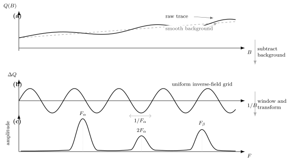
A defensible transform keeps the raw observable $Q(B)$, a declared smooth background, the residual on a uniform $1/B$ grid, the field window, and the windowed frequency spectrum. Harmonics such as $2F_\alpha$ and distinct orbits such as $F_\beta$ require separate assignments; a peak label is not itself a pocket identification.

Background removal

Write the measured channel as

$$Q(B) = Q_{\mathrm{bg}}(B) + \Delta Q(B).$$

$Q_{\mathrm{bg}}$ may be estimated by a low-order polynomial, spline, physically motivated smooth model, or low-pass procedure. No method is neutral. An overly flexible background can absorb low-frequency oscillations; an overly rigid one leaves curvature that appears as spectral weight near zero frequency. A robust analysis repeats the extraction across reasonable background families and reports which peaks and phases survive.

Never discard the raw trace. Publish or archive the background function, its parameters, the exact fit interval, masked regions, and the residual before and after any filtering. A Fourier spectrum alone is not reproducible evidence.

Uniform inverse-field sampling

Oscillations of one ideal orbit take the schematic form

$$\Delta Q(B) \propto \cos\!\left( 2\pi\frac{F}{B} + \phi \right).$$

Define $x=1/B$. Data acquired uniformly in $B$ are nonuniform in $x$ and should be interpolated or analyzed with a method that handles nonuniform samples. Interpolation should not invent resolution; its grid spacing only needs to support the highest retained frequency under a documented sampling criterion.

For a field interval $B_{\min}\leq B\leq B_{\max}$, the inverse-field span is

$$\Delta x = \frac{1}{B_{\min}} - \frac{1}{B_{\max}}.$$

The characteristic Fourier resolution is

$$\delta F \gtrsim \frac{1}{\Delta x}.$$

Window functions reduce spectral leakage at the price of broadening peaks and changing amplitude normalization. Zero-padding makes a plotted spectrum smoother but does not increase the independent information or resolve two frequencies closer than the finite-window limit.

A practical transform workflow

1. Choose the field interval before looking for a preferred peak or phase.
2. Mask transitions, contact jumps, pulse artifacts, and hysteretic regions with recorded criteria.
3. Fit several defensible smooth backgrounds.
4. Convert to $x=1/B$ and resample uniformly, or use a validated nonuniform transform.
5. Apply and name a window function.
6. Transform with an explicit amplitude normalization.
7. repeat the analysis over neighboring field windows and background choices;
8. fit the time-domain residual as a cross-check when peaks overlap or phase matters.

A moving-window transform can reveal field-dependent frequencies, but its frequency and field resolutions trade against each other. Apparent peak drift can also arise from beating, amplitude modulation, changing background, or a short window.

Lifshitz–Kosevich Analysis

For a conventional three-dimensional Fermi liquid with a well-defined closed orbit, a useful schematic form for harmonic $p$ is

$$\begin{aligned} \Delta Q_p(B,T) ={}& C_p B^\lambda R_{T,p}R_{D,p}R_{S,p} \\ &\times \cos\!\left( 2\pi p\frac{F}{B} + \phi_p \right), \end{aligned}$$

with

$$\begin{aligned} R_{T,p} &= \frac{X_p}{\sinh X_p}, \\ X_p &= \alpha p \frac{m_c}{m_e} \frac{T}{B}, \\ R_{D,p} &= \exp\!\left[ -\alpha p \frac{m_c}{m_e} \frac{T_D}{B} \right], \\ \alpha &= \frac{2\pi^2k_{\mathrm B}m_e}{e\hbar} \\ & = 14.694\ \mathrm{T\,K^{-1}}. \end{aligned}$$

$C_p$, the field power $\lambda$, and the phase $\phi_p$ depend on dimensionality, observable, orbit curvature, and convention. This compact expression is a fit scaffold, not a universal waveform.

Cyclotron mass from temperature damping

At fixed orbit, angle, and field window, fit the temperature dependence to $R_{T,p}$. Fourier amplitudes average a field-dependent signal over the window. A common approximation evaluates $R_T$ at the midpoint in inverse field,

$$\frac{1}{B_{\mathrm{eff}}} = \frac{1}{2} \left( \frac{1}{B_{\min}} + \frac{1}{B_{\max}} \right).$$

That approximation should be tested by integrating the modeled field dependence through the actual background, interpolation, and window pipeline. Reusing different field windows at different temperatures can bias the fitted mass. So can an unresolved doublet whose components have different masses.

The measured $m_c$ is the energy derivative of the orbit area. It need not equal a local band-curvature mass, an optical mass, or a thermodynamic density-of-states mass. In an interacting metal, it includes quasiparticle renormalization along that orbit.

Dingle damping and quantum lifetime

The Dingle temperature is conventionally related to a quantum lifetime by

$$T_D = \frac{\hbar} {2\pi k_{\mathrm B}\tau_q}.$$

After dividing out the known thermal and field prefactors, a Dingle plot tests exponential damping versus $1/B$. Curvature in that plot can indicate field-dependent scattering, unresolved frequencies, magnetic breakdown, spin interference, an incorrect field prefactor, or failure of the assumed background. A fitted straight line is meaningful only if these alternatives are constrained.

The corresponding quantum mobility scale is

$$\mu_q = \frac{e\tau_q}{m_c}.$$

It is not generally the Hall or transport mobility. Reporting all three as interchangeable obscures real information about scattering.

Spin damping

For a simple orbit with an effective $g$ factor and negligible complications, the spin reduction factor is often written

$$R_{S,p} = \cos\!\left( \frac{\pi p g^*m_c} {2m_e} \right).$$

A zero of $R_{S,p}$ can suppress the fundamental and make a harmonic appear dominant. In tilted, spin–orbit-coupled, magnetic, or multiband systems, both $g^*$ and $m_c$ can depend on angle and field, and the scalar formula may be inadequate. An absent frequency at one angle is therefore not proof that the orbit disappears.

Angular Dependence and Fermi-Surface Geometry

Rotate the field relative to crystallographic axes and track each peak continuously. For an ideal two-dimensional cylindrical Fermi surface,

$$F(\theta) \lvert\cos\theta\rvert \approx F(0),$$

where $\theta$ is measured from the cylinder axis. Deviations can reveal warping, a closed three-dimensional pocket, reconstruction, or a mistaken angle zero. Near $\theta=90^\circ$, the ideal expression diverges and small alignment errors are amplified.

Three-dimensional pockets generally produce several extremal branches whose frequencies can merge, split, or exchange amplitude with angle. Branch tracking should use frequency, mass, amplitude, and continuity together. Assigning each isolated peak independently at every angle can create artificial discontinuities.

Torque amplitude also contains an angular derivative of the orbit frequency. A branch can become weak where $dF/d\theta$ is small, even though the orbit remains present. Comparing torque, magnetization, and transport prevents detector-specific zeros from being mistaken for topological changes.

Fermi-Surface Reconstruction

Translation-symmetry breaking with wavevector $\mathbf Q$ folds bands into a reduced Brillouin zone. Hybridization at crossings can replace a large unreconstructed surface with smaller electron and hole pockets. Quantum oscillations can then reveal new frequencies and masses that are difficult to infer from smooth transport alone.

The strongest reconstruction case combines:

• a thermodynamic or diffraction signature of the ordering wavevector;
• frequency changes across the same control parameter;
• angle dependence consistent with reconstructed pockets;
• carrier-sign or compensation constraints from Hall and thermoelectric response;
• a band-folding calculation using the observed symmetry and order;
• accounting for all required degeneracies and plausible unobserved heavy pockets.

Small frequencies alone do not identify the order responsible for them. They can arise from an unreconstructed small pocket, surface states, bilayer splitting, warping, or a minority phase.

Magnetic breakdown and combination frequencies

At high field, a quasiparticle can tunnel across a small momentum-space gap between neighboring semiclassical orbits. A common leading probability has the form

$$P_{\mathrm{MB}} \sim \exp\!\left( -\frac{B_0}{B} \right),$$

where $B_0$ depends on the local gap and velocities. Breakdown can generate large composite orbits, sum and difference frequencies, and field-dependent redistribution of amplitude. Harmonics, chemical-potential oscillations, and nonlinear mixing can generate related spectral structures without corresponding to independent pockets.

Before counting every Fourier peak as a Fermi-surface sheet, test frequency arithmetic, harmonic mass scaling, field dependence, and the expected breakdown network. Conversely, a reconstructed pocket can be invisible because it is heavy or strongly scattered. Luttinger counting from observed frequencies is incomplete until missing sheets and degeneracies are bounded.

Berry Phase and Landau-Fan Cautions

For one isolated nondegenerate orbit in the simplest semiclassical limit,

$$\gamma = \frac{1}{2} - \frac{\Phi_{\mathrm B}}{2\pi},$$

so the Berry phase $\Phi_{\mathrm B}$ shifts the orbit quantization. This elegant relation motivates phase analysis, but the phase measured in an oscillatory observable generally also contains:

• a three-dimensional stationary-phase or Maslov correction, commonly $0$ in an ideal two-dimensional limit and $\pm1/8$ for simple three-dimensional extremal orbits;
• Zeeman splitting and spin-dependent amplitude reversals;
• orbital magnetic-moment corrections;
• observable-dependent derivatives and conductivity-tensor inversion;
• warping, magnetic breakdown, and chemical-potential oscillations;
• multiple close frequencies or unresolved harmonics;
• a convention-dependent choice of which maxima or minima receive integer indices.

Modern semiclassical theory combines geometric phase, orbital moment, and spin transport around the orbit. A fitted fundamental phase is therefore not generally a direct Berry phase, and a near-$\pi$ value is not by itself a unique signature of a Dirac or Weyl band.

Landau-fan construction

A Landau fan plots assigned index $n$ against $1/B_n$ for selected extrema and fits a line. A defensible fan requires:

1. deriving the extrema-to-index rule for the measured observable and tensor regime;
2. tracking one orbit without switching branches;
3. resolving spin splitting or modeling it;
4. using enough periods that slope and intercept are not strongly covariant;
5. propagating uncertainty in field, extrema location, and index assignment;
6. testing the fit against the full oscillatory waveform.

Extrapolating an intercept from only a few high-field levels is especially fragile. A one-index shift leaves the frequency nearly unchanged but changes the intercept by one. Background choices can move broad extrema, while unresolved beating can shift them nonuniformly. The safer hierarchy is: determine frequency and orbit geometry first, constrain dimensional and spin corrections independently, then fit the complete field-domain signal under competing phase models.

Uncertainty and Reproducibility

A quantum-oscillation uncertainty budget should separate experimental, processing, and model contributions.

Contribution	Examples	Useful checks
field coordinate	calibration, hysteresis, pulse timing	reference probe, both sweep directions
temperature	thermometer lag, eddy heating, magnetocaloric response	current and sweep-rate series, pulse-branch comparison
angle	mount offset, backlash, field-induced rotation	symmetry orientations, bidirectional rotation
raw observable	contact mixing, cantilever calibration, lock-in phase	lead reversal, calibration standard, bandwidth test
background	polynomial order, spline knots, mask boundaries	alternate backgrounds, synthetic-signal recovery
transform	interpolation, window, normalization, finite span	neighboring windows, time-domain fit
orbit model	dimension, harmonics, spin, breakdown, chemical potential	competing fits, angle and temperature dependence

Parameter covariance matters. Frequency and phase correlate over a short inverse-field window; mass correlates with the chosen effective field; Dingle temperature correlates with the field prefactor and background; two nearby amplitudes correlate below the transform resolution. Report confidence regions or covariance matrices when these parameters support a physical claim.

A reusable data release includes raw signed traces, calibration metadata, thermometer and angle records, processing code, background alternatives, masks, transform conventions, fit residuals, and machine-readable parameter tables. Plot images are not a substitute for the underlying traces.

Common Mistakes

• Fourier transforming data uniform in $B$ as though they were uniform in $1/B$.
• Treating zero-padding as improved frequency resolution.
• Choosing the background or field window because it gives the desired peak.
• Calling every peak an independent pocket without checking harmonics or magnetic breakdown.
• Inferring electron or hole sign from frequency alone.
• Fitting masses over different field windows at different temperatures.
• Equating Dingle, transport, and Hall mobilities.
• Assigning Landau indices to resistance extrema without tensor inversion and a forward model.
• Reading a Berry phase directly from one intercept.
• Interpreting a missing branch as proof that the Fermi-surface sheet vanished.

Exercises

1. Orbit area and circular wavevector

A fundamental frequency is $F=500\,\mathrm T$. Find the extremal area in $\mathrm m^{-2}$ and $\text{\AA}^{-2}$. If the cross section is circular, estimate $k_{\mathrm F}$. Use $e=1.602\times10^{-19}\,\mathrm C$ and $\hbar=1.055\times10^{-34}\,\mathrm{J\,s}$.

Solution

The Onsager relation gives

$$\begin{aligned} A_{\mathrm{ext}} &= \frac{2\pi e}{\hbar}F \\ &= 4.77\times10^{18}\,\mathrm m^{-2} \\ &= 0.0477\,\text{\AA}^{-2}. \end{aligned}$$

For a circular orbit,

$$k_{\mathrm F} = \sqrt{\frac{A_{\mathrm{ext}}}{\pi}} = 0.123\,\text{\AA}^{-1}.$$

The frequency determines an extremal cross section. Circularity and the assignment to a particular pocket are additional assumptions.

2. Finite-window resolution

Data are analyzed from $10$ to $20\,\mathrm T$. Estimate the Fourier resolution. Can this window cleanly resolve peaks at $300$ and $312\,\mathrm T$? Would zero-padding settle the question?

Solution

The inverse-field span is

$$\Delta x = \frac{1}{10\,\mathrm T} - \frac{1}{20\,\mathrm T} = 0.050\,\mathrm T^{-1}.$$

Thus

$$\delta F \gtrsim \frac{1}{\Delta x} = 20\,\mathrm T.$$

The proposed peaks are separated by only $12\,\mathrm T$, below this characteristic resolution. Their sum can produce a broadened or window-dependent feature, but the window does not independently resolve them. Zero-padding only interpolates the discrete spectrum; it cannot add the missing inverse-field span.

3. Thermal damping

For $m_c=0.50m_e$ and $B_{\mathrm{eff}}=15\,\mathrm T$, calculate the fundamental $R_T$ at $T=1.0\,\mathrm K$ and $5.0\,\mathrm K$.

Solution

Using $X=14.694(m_c/m_e)T/B$,

$$\begin{aligned} X(1\,\mathrm K) &= 0.490, \\ R_T(1\,\mathrm K) &= \frac{0.490}{\sinh(0.490)} \approx 0.961, \\ X(5\,\mathrm K) &= 2.45, \\ R_T(5\,\mathrm K) &= \frac{2.45}{\sinh(2.45)} \approx 0.426. \end{aligned}$$

The amplitude falls by more than a factor of two. A mass fit should use all temperatures and propagate the uncertainty in field-window averaging rather than infer $m_c$ from one ratio.

4. Dingle scale and quantum mobility

An orbit has $m_c=0.20m_e$ and $T_D=8.0\,\mathrm K$. Find $R_D$ at $12\,\mathrm T$, $\tau_q$, and $\mu_q$. Use $m_e=9.109\times10^{-31}\,\mathrm{kg}$.

Solution

For the fundamental,

$$\begin{aligned} \alpha \frac{m_c}{m_e} \frac{T_D}{B} &= 1.96, \\ R_D &= e^{-1.96} = 0.141. \end{aligned}$$

The lifetime is

$$\tau_q = \frac{\hbar}{2\pi k_{\mathrm B}T_D} = 1.52\times10^{-13}\,\mathrm s.$$

Therefore

$$\begin{aligned} \mu_q &= \frac{e\tau_q}{0.20m_e} \\ &= 0.134\,\mathrm{m^2\,V^{-1}\,s^{-1}} \\ &= 1.34\times10^3\, \mathrm{cm^2\,V^{-1}\,s^{-1}}. \end{aligned}$$

This is a quantum mobility inferred from level broadening. It need not match a transport or Hall mobility.

5. Angular test of a cylinder

A quasi-two-dimensional orbit has $F(0)=200\,\mathrm T$. What does an ideal cylindrical model predict at $\theta=60^\circ$? The measured branch is instead $350\,\mathrm T$. Name three possible interpretations.

Solution

For an ideal cylinder,

$$F(60^\circ) = \frac{200\,\mathrm T} {\lvert\cos60^\circ\rvert} = 400\,\mathrm T.$$

The lower observed frequency could reflect Fermi-surface warping or a closed three-dimensional pocket, an angle-zero or sample-alignment error, or incorrect tracking of the branch. Reconstruction and field-dependent band structure are further possibilities. A single angle cannot distinguish them; follow the branch continuously and compare with a geometric model and an independent angle calibration.

6. What does a fan intercept establish?

A linear Landau-fan fit from six extrema gives an intercept consistent with zero. An analyst calls this proof of a $\pi$ Berry phase. List the minimum checks required before that statement is defensible.

Solution

The analyst must establish which measured tensor component was fitted and whether integer indices belong to maxima or minima; constrain the two- or three-dimensional phase correction; resolve or model Zeeman splitting and spin zeros; include orbital-moment corrections where relevant; exclude unresolved beating, harmonics, and magnetic breakdown; test background and field-window dependence; propagate slope-intercept covariance and index uncertainty; and compare the fan with a full waveform fit.

Even after those checks, the result is a model-dependent phase constraint. In a general multiband solid, the observable phase contains more than the Berry phase. A zero intercept is therefore not universal proof of a Dirac band or topological protection.

Research Status

• Established: Onsager frequency-area correspondence for closed semiclassical orbits; Lifshitz–Kosevich thermal damping in its regime of validity; Shubnikov–de Haas and de Haas–van Alphen measurements as Fermi-surface probes; finite inverse-field resolution.
• Model dependent: pocket assignment, field prefactors, Dingle extraction, effective $g$ factors, background models, magnetic-breakdown networks, and carrier counting from the observed subset of frequencies.
• Active: quantum oscillations in non-Fermi liquids, very low-density semimetals, superconducting states, moiré systems, putative correlated insulators, and regimes with strong chemical-potential oscillation or interaction-driven frequency shifts.
• Not established by one spectrum or intercept: a complete Fermi surface, carrier sign, one reconstruction mechanism, a unique Berry phase, or topological protection.

Connections

• Fermi Surface derives orbit geometry, extremal-area selection, the Onsager relation, and cyclotron mass.
• Angle-Resolved Photoemission Spectroscopy provides the complementary surface-sensitive occupied dispersion, orbital selection, and line-shape view of the Fermi surface.
• Landau Levels develops orbital quantization, degeneracy, and level crossings in uniform magnetic fields.
• Effective Mass distinguishes the several masses that appear in band structure, optics, thermodynamics, and oscillations.
• Transport Measurements supplies the four-terminal, current-reversal, heating, sweep, and uncertainty checks for Shubnikov–de Haas data.
• Hall Measurements develops simultaneous transverse-voltage reduction and explains when Hall sign or density can constrain an orbit assignment.
• Berry Phase defines geometric phase, gauge invariance, and adiabatic holonomy.
• Charge and Spin Density Waves develops translation-symmetry breaking and the band folding that can reconstruct a Fermi surface.
• Weyl and Dirac Semimetals discusses nodal-band orbit structure and why a phase offset alone is not a topology test.
• Two-Dimensional Electron Gases connects oscillations to filling factor, spin splitting, and quantum Hall regimes.
• Error Estimates supplies regression, covariance, conditioning, and model-discrepancy tools.

Further Reading

• D. Shoenberg remains the comprehensive monograph on orbit geometry, experimental methods, magnetic breakdown, Dingle analysis, phase, and spin splitting.
• L. Onsager and I. M. Lifshitz with A. M. Kosevich give the foundational frequency and amplitude theory.
• A. Alexandradinata et al. formulate modern phase offsets including geometric, orbital, spin, and symmetry information.
• A. A. Taskin with Y. Ando and A. R. Wright with R. H. McKenzie show why realistic Dirac-band fan analysis is subtler than reading an intercept.
• Quantum-oscillation studies of underdoped cuprates provide an instructive reconstruction case in which small pockets are well established but their complete microscopic interpretation requires several probes.

References

1. L. Onsager, “Interpretation of the de Haas–van Alphen Effect”, Philosophical Magazine 43, 1006–1008 (1952).
2. I. M. Lifshitz and A. M. Kosevich, “Theory of Magnetic Susceptibility in Metals at Low Temperatures”, Soviet Physics JETP 2, 636–645 (1956).
3. R. B. Dingle, “Some Magnetic Properties of Metals. II. The Influence of Collisions on the Magnetic Behaviour of Large Systems”, Proceedings of the Royal Society A 211, 517–525 (1952).
4. D. Shoenberg, Magnetic Oscillations in Metals, Cambridge University Press (1984).
5. G. P. Mikitik and Yu. V. Sharlai, “Manifestation of Berry’s Phase in Metal Physics”, Physical Review Letters 82, 2147–2150 (1999).
6. A. A. Taskin and Y. Ando, “Berry Phase of Nonideal Dirac Fermions in Topological Insulators”, Physical Review B 84, 035301 (2011).
7. A. R. Wright and R. H. McKenzie, “Quantum Oscillations and Berry’s Phase in Topological Insulator Surface States with Broken Particle-Hole Symmetry”, Physical Review B 87, 085411 (2013).
8. A. Alexandradinata, C. Wang, W. Duan, and L. Glazman, “Revealing the Topology of Fermi-Surface Wave Functions from Magnetic Quantum Oscillations”, Physical Review X 8, 011027 (2018).
9. N. Doiron-Leyraud et al., “Quantum Oscillations and the Fermi Surface in an Underdoped High-$T_c$ Superconductor”, Nature 447, 565–568 (2007).
10. E. A. Yelland et al., “Quantum Oscillations in the Underdoped Cuprate $\mathrm{YBa_2Cu_4O_8}$”, Physical Review Letters 100, 047003 (2008).
11. A. F. Bangura et al., “Small Fermi Surface Pockets in Underdoped High Temperature Superconductors: Observation of Shubnikov–de Haas Oscillations in $\mathrm{YBa_2Cu_4O_8}$”, Physical Review Letters 100, 047004 (2008).
12. A. Carrington, “Quantum Oscillation Studies of the Fermi Surface of Iron-Pnictide Superconductors”, Reports on Progress in Physics 74, 124507 (2011).
13. Joint Committee for Guides in Metrology, Evaluation of Measurement Data: Guide to the Expression of Uncertainty in Measurement, JCGM 100:2008.

Summary

• Quantum oscillations are detector-dependent modulations generated when Landau-quantized closed orbits cross the chemical potential.
• Frequency robustly constrains an extremal orbit area, while carrier sign and full three-dimensional geometry require additional evidence.
• Shubnikov–de Haas analysis must respect the conductivity tensor; de Haas–van Alphen analysis avoids that tensor ambiguity but retains damping, spin, and torque-specific effects.
• Background choice, uniform $1/B$ sampling, windowing, and finite-span resolution are part of the result and must be reported.
• Lifshitz–Kosevich temperature damping yields a cyclotron mass; Dingle damping yields a model-dependent quantum lifetime distinct from the transport lifetime.
• Reconstruction claims require symmetry and multi-probe closure, and phase claims require a complete semiclassical and detector model rather than one fan intercept.