Pump–Probe Spectroscopy

Pump–probe spectroscopy asks how a material changes after a controlled excitation. A pump pulse prepares a nonequilibrium state; a delayed probe pulse measures an observable; repeating the experiment while scanning the delay produces a time-resolved differential signal. The method can follow carrier redistribution, order-parameter suppression, energy transfer, coherent lattice motion, metastable switching, and driven states on time scales from attoseconds to seconds.

The word time-resolved does not make the measured trace a movie of one microscopic variable. The detector records a probe-dependent projection of a repeatedly prepared, spatially inhomogeneous, open system. Converting that record into a carrier temperature, quasiparticle density, phonon coordinate, gap, or transient phase requires a forward model and controls for pulse overlap, heating, penetration depth, repetition rate, matrix elements, and recovery between shots.

A useful evidence ladder is:

1. detector record: photodiode voltage, camera counts, electron counts, or emitted field versus nominal delay;
2. differential observable: $\Delta R/R$, $\Delta T/T$, photoelectron intensity, diffraction intensity, or complex conductivity after normalization and artifact treatment;
3. material response: a change in dielectric function, occupation, spectral function, lattice coordinate, symmetry channel, or order-sensitive response under an explicit model;
4. nonequilibrium state: a reproducible distribution or collective configuration with calibrated excitation density, depth profile, and lifetime;
5. phase-level claim: evidence for transient order, symmetry, rigidity, topology, or metastability that survives alternative explanations and is corroborated by independent observables.

The last step is deliberately demanding. A differential optical feature can be excellent evidence for a changed optical response without, by itself, establishing a new thermodynamic phase.

Canonical Scope

This page is the canonical home for pump–probe practice in quantum materials: absorbed-fluence and penetration-depth accounting, time-resolved reflectivity, time-resolved angle-resolved photoemission, coherent phonon readout, phenomenological relaxation models, light-induced-state claims, and the controls needed to interpret them.

Ultrafast Spectroscopy Overview owns general pulse language, Fourier-limited time–bandwidth relations, cross-correlation, instrument-response convolution, molecular wave packets, multidimensional spectroscopy, and attosecond methods. Angle-Resolved Photoemission Spectroscopy owns equilibrium ARPES kinematics, analyzers, matrix elements, and spectral-function interpretation. Quenches owns idealized quench protocols, injected energy, return amplitudes, and correlation spreading in model systems. Quantum Thermalization owns ensemble claims and the distinction between dephasing, local equilibration, and thermalization.

Equilibrium optical constants and complex low-energy conductivity belong to Terahertz and Infrared Probes. The present page uses those quantities as delayed observables and concentrates on what the pump changes.

Nonequilibrium Excitation

Repeated preparation, not passive observation

Most pump–probe experiments are stroboscopic. At every laser shot, a nominally identical pump prepares the sample, and one probe delay is sampled. A delay scan is assembled from many independently prepared trajectories. The measured point at delay $t_d$ is therefore an average over pulses, beam profiles, illuminated domains, detector integration time, and any slow drift:

$$\overline{S}(t_d) = \frac{1}{N} \sum_{j=1}^{N} S_j(t_d).$$

This construction assumes reproducibility. If the material switches irreversibly, ages, accumulates defects, drifts thermally, or recovers more slowly than the pulse period, points acquired later in the scan need not represent the same initial state. Delay randomization, pump chopping, alternating reference shots, bidirectional scans, and explicit reset protocols test that assumption.

Let the repetition rate be $f_{\mathrm{rep}}$. Full recovery requires more than the decay of the fastest optical transient. Electronic occupation, lattice temperature, strain, trapped charge, domains, and the cryostat mount can recover on very different time scales. A signal that is unchanged when $f_{\mathrm{rep}}$ is varied at fixed absorbed fluence is less likely to be dominated by cumulative heating, although it does not exclude single-pulse heating.

Incident fluence, absorbed fluence, and peak field

For pulse energy $U_p$ and a spatial fluence profile $F(x,y)$,

$$U_p = \int F(x,y)\,dx\,dy.$$

Quoting $U_p$ divided by an ill-defined spot area is not enough. A Gaussian beam with $1/e^2$ intensity radius $w$ has

$$F(r) = F_0 e^{-2r^2/w^2}, \qquad F_0 = \frac{2U_p}{\pi w^2}.$$

Thus the peak fluence is twice $U_p/(\pi w^2)$. Authors should state whether a radius is a standard deviation, a full width at half maximum, a $1/e$ radius, or a $1/e^2$ radius.

For a thick, homogeneous sample at normal incidence with negligible transmission, a first absorption estimate is

$$F_{\mathrm{abs}} = (1-R_p)F_{\mathrm{inc}},$$

where $R_p$ is the pump reflectance at the pump photon energy and polarization. The associated depth-dependent deposited energy density is

$$u(z) = F_{\mathrm{abs}}\alpha_p e^{-\alpha_p z},$$

with pump absorption coefficient $\alpha_p$. If a fraction $\eta$ of absorbed photons produces the excitation being counted, then

$$n_{\mathrm{ex}}(z) = \eta \frac{u(z)}{\hbar\omega_p}.$$

These formulas are estimates, not universal calibrations. Thin films and heterostructures require multilayer absorption; anisotropic crystals require polarization-dependent optical constants; resonant saturation, nonlinear absorption, bleaching, and pump-induced changes can invalidate a linear Beer–Lambert profile.

For field-driven experiments, fluence alone can hide the relevant control parameter. For a plane wave in vacuum, a peak intensity $I_0$ corresponds to

$$E_0 = \sqrt{\frac{2I_0}{c\varepsilon_0}},$$

before reflection, focusing, pulse-envelope, and in-medium corrections. Carrier injection often scales with absorbed photon number, whereas tunneling, nonlinear polarization, coherent control, and strong-field dressing can depend sensitively on peak electric field and carrier-envelope conditions.

Spatial averaging and depth mismatch

The pump and probe almost never weight the same volume. If the local response is $\Delta s(z,t)$ and the probe sensitivity is $W_{\mathrm{pr}}(z)$, a useful schematic model is

$$\Delta S_{\mathrm{meas}}(t) = \frac{ \int_0^\infty W_{\mathrm{pr}}(z)\Delta s(z,t)\,dz }{ \int_0^\infty W_{\mathrm{pr}}(z)\,dz }.$$

For $\Delta s(z,t)=\Delta s_0(t)e^{-\alpha_pz}$ and $W_{\mathrm{pr}}(z)=e^{-\alpha_{\mathrm{pr}}z}$,

$$\Delta S_{\mathrm{meas}}(t) = \Delta s_0(t) \frac{\alpha_{\mathrm{pr}}}{ \alpha_p+\alpha_{\mathrm{pr}} }.$$

A shallow pump and deep probe therefore dilute the surface response. The same issue appears laterally because both beams have finite profiles and the probe integrates a continuum of local fluences. A sharp local threshold can become a smooth measured crossover. Reporting only the peak fluence obscures this averaging.

The pump spot is commonly made larger than the probe spot, but a size ratio alone does not prove uniform excitation. Beam images at the sample, incidence-angle corrections, astigmatism, pointing stability, and the probe-weighted fluence distribution are all relevant.

Heating and nonthermal distributions

Immediately after optical absorption, the electronic distribution need not be describable by a temperature. Electron–electron scattering may establish a Fermi-like distribution before substantial energy reaches phonons, but that hierarchy is material-, energy-, and fluence-dependent. A fitted electronic temperature is meaningful only when the measured distribution is consistent with one over a stated energy range.

The maximum adiabatic temperature rise from a deposited energy density can be estimated from

$$u = \int_{T_0}^{T_f} C_V(T)\,dT,$$

where $C_V$ is the relevant volumetric heat capacity. At early times, the participating heat capacity may be electronic or mode selective; at long times it approaches that of the heated sample volume and environment. Comparing a transient spectrum with an equilibrium temperature series is valuable, but equality of one spectral feature does not prove full thermal equilibrium.

Average absorbed power provides a separate heat load:

$$P_{\mathrm{abs}} = f_{\mathrm{rep}} \int F_{\mathrm{abs}}(x,y)\,dx\,dy.$$

Varying fluence and repetition rate independently helps distinguish a response tied to energy per pulse from one tied to average heating. Base-temperature thermometry can still miss a hotter microscopic illuminated region.

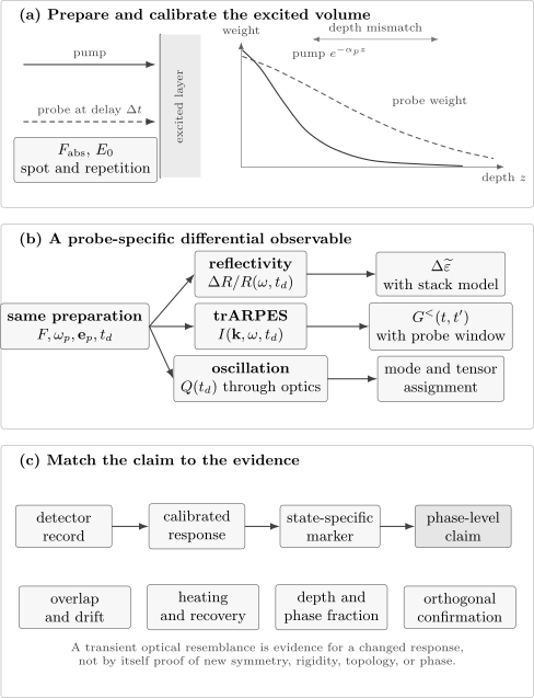
A pump–probe result passes through three distinct layers: a nonuniform, repeatedly prepared excitation; a probe-specific differential observable; and an inference whose strength depends on controls for overlap, heating, depth mismatch, recovery, and alternative mechanisms.

Time-Resolved Reflectivity

The measured ratio

In a common implementation, the pump is modulated and a photodiode plus lock-in amplifier measures the pump-induced change in reflected probe power. With $R_0$ the unpumped reflectance,

$$\frac{\Delta R}{R}(t_d) = \frac{ R_{\mathrm{pumped}}(t_d)-R_0 }{ R_0 }.$$

This ratio suppresses some laser noise, but it is not itself a microscopic population. At normal incidence on a homogeneous semi-infinite medium,

$$r = \frac{1-\widetilde n}{1+\widetilde n}, \qquad R = \lvert r\rvert^2,$$

where $\widetilde n=n+i\kappa$ is the complex refractive index. For a small pump-induced change,

$$\frac{\Delta R}{R} \simeq 2\operatorname{Re} \left( \frac{\Delta r}{r} \right).$$

The measured scalar therefore mixes the real and imaginary changes of $\widetilde n$, and hence of the complex dielectric function. The sign of $\Delta R/R$ is not universally the sign of carrier density, gap suppression, or temperature.

In a film, substrate, or heterostructure, $r$ is a multilayer amplitude containing propagation phases and interface coefficients. The same local $\Delta\varepsilon$ can give opposite $\Delta R$ at different film thicknesses or probe wavelengths. A quantitative inversion should propagate a depth-dependent perturbation through a multilayer optical model rather than assign each exponential component directly to a microscopic species.

Spectral and polarization information

A single-color trace records one projection of the transient dielectric function. Broadband probing instead measures

$$\frac{\Delta R}{R}(\omega,t_d),$$

which can separate a shifted resonance, broadened line, transferred spectral weight, and nearly featureless background. Polarization-resolved measurements test anisotropy and symmetry. Comparison with equilibrium temperature, magnetic field, strain, or doping series helps identify whether the transient spectrum follows a known state manifold.

Global analysis can share physically common parameters across wavelengths and delays, but only if the model is identifiable. Singular-value decomposition can estimate the number of significant spectral components; it does not tell which component is a quasiparticle, phonon, or order parameter.

Time zero and coherent artifacts

Near temporal overlap, the pump and probe can mix through cross-phase modulation, two-photon absorption, stimulated Raman processes, scattered pump light, nonlinear response of a substrate, or electronic interference. Such a coherent artifact may be narrower than the material relaxation and may change with polarization or detection geometry.

The nominal translation-stage zero is not necessarily the sample time zero. Broadband probes have wavelength-dependent group delay, or chirp, so each detector pixel can correspond to a different effective delay. A reliable analysis measures or fits the instrument response, corrects the delay surface, and excludes or explicitly models overlap-dominated data. A sub-pulse-width spike should not be promoted to an intrinsic decay constant merely because an exponential fit accepts it.

Relaxation components are not identities

Multiexponential fitting,

$$\frac{\Delta R}{R}(t) = \sum_j A_j e^{-t/\tau_j} +C,$$

can compress a dataset, but the labels fast carriers, phonon cooling, and recombination do not follow from the fit. Distributed relaxation rates, diffusion, nonlinear kinetics, a changing spectrum, and convolution with the instrument response can all produce effective exponentials. Report parameter covariance, fit window, residuals, and whether the same parameters describe fluence, temperature, wavelength, and polarization dependences.

Time-Resolved ARPES

What the probe adds

Time-resolved ARPES, commonly abbreviated trARPES, pumps the material and photoemits electrons with a delayed ultraviolet or extreme-ultraviolet probe. Compared with equilibrium ARPES, it can access transiently occupied states above the chemical potential, follow momentum-resolved population decay, track band and gap changes, and observe coherent energy or momentum shifts.

The equilibrium relation between intensity, matrix elements, spectral function, and occupation remains a useful guide,

$$I(\mathbf k,\omega) \propto \lvert M\rvert^2 A(\mathbf k,\omega) f(\omega),$$

but out of equilibrium there need not be a time-independent spectral function multiplied by a Fermi function. A gauge-consistent theoretical description uses a two-time lesser Green function sampled by the finite probe envelope. Schematically,

$$\begin{aligned} I(\mathbf k,\omega,t_0) \propto{}& -i\lvert M\rvert^2 \int dt\,dt'\, s(t-t_0)s(t'-t_0) \\ &\times e^{i\omega(t-t')} G_{\mathbf k}^{<}(t,t'). \end{aligned}$$

Here $s(t-t_0)$ is the probe envelope and $G_{\mathbf k}^{<}$ contains occupied single-particle correlations. The finite temporal window means that a trARPES frame is not an instantaneous spectrum. When the system changes substantially during the probe pulse, energy and time cannot be assigned independently.

Resolution and identifiability

Shortening a transform-limited probe improves temporal resolution but broadens its spectrum. For Gaussian intensity profiles,

$$\Delta\nu\,\Delta t \geq 0.441.$$

The experiment also convolves pump duration, probe duration, timing jitter, analyzer resolution, photon bandwidth, and space-charge broadening. A claimed subcycle or few-femtosecond material response must be supported by an independently measured cross-correlation and an analysis compatible with the probe window.

Population above the chemical potential does not by itself reveal whether a band moved, a gap closed, a self-energy changed, or occupation was transferred into a pre-existing state. Energy-distribution and momentum-distribution cuts, full two-dimensional fits, equilibrium controls, and matrix-element variation with photon energy and polarization help separate those possibilities.

trARPES-specific artifacts

Several effects can imitate electronic-structure dynamics:

• space charge: electrons emitted in one pulse repel one another, shifting and broadening the spectrum in a count-rate-dependent way;
• surface photovoltage: photoexcited carriers modify near-surface band bending, shifting spectral energies with material- and time-dependent recovery;
• pump-induced vacuum fields: emitted charge and the pump field can accelerate outgoing photoelectrons, producing delay-dependent energy or momentum shifts;
• laser-assisted photoemission: pump–probe overlap can dress the outgoing final state and create sidebands that are not intrinsic Floquet bands of the solid;
• chemical-potential and reference drift: sample charging, contact potentials, and analyzer drift can mimic a changing band energy;
• matrix-element dynamics: altered orbital character, polarization geometry, and final-state resonance can change intensity without a proportional change in occupation.

Count-rate scans, pump-polarization controls, delay scans extending far beyond overlap, grounded metallic references, photon-energy dependence, and explicit final-state calculations are therefore part of the measurement, not optional embellishments.

Coherent Phonons

A driven coordinate

An ultrashort pump can launch a phase-coherent normal coordinate $Q$. A compact phenomenological equation that includes impulsive and displacive limits is

$$\ddot Q +2\Gamma\dot Q +\Omega^2 \left[ Q-Q_{\mathrm{eq}}(t) \right] = \frac{F_{\mathrm{ISRS}}(t)}{M}.$$

Here $\Omega$ is the mode frequency, $\Gamma$ its damping rate, $Q_{\mathrm{eq}}(t)$ a pump-shifted equilibrium coordinate, and $F_{\mathrm{ISRS}}$ an impulsive stimulated-Raman force. A suddenly displaced equilibrium produces a cosine-like oscillation about the new position; an impulsive force produces a sine-like response in the ideal limits.

Reflectivity detects the coordinate through the optical susceptibility. To leading order,

$$\left( \frac{\Delta R}{R} \right)_{\mathrm{osc}} \simeq \frac{\partial\ln R}{\partial Q} Q(t).$$

The derivative depends on probe photon energy and polarization, so the same lattice trajectory can appear with different amplitude or phase in different optical channels. Finite pump duration, chirp, resonant absorption, mixed driving mechanisms, anharmonicity, and propagation also change the phase. Phase alone is therefore not a decisive classifier of displacive excitation versus impulsive stimulated Raman scattering.

Optical and acoustic modes

Zone-center Raman-active optical phonons are natural coherent modes because visible photons transfer little momentum. Their frequencies can be compared with equilibrium Raman and Optical Spectroscopy and eigenvectors from Phonons. Pump-polarization and crystal-symmetry dependence test the driving tensor, while probe-polarization dependence tests the detection tensor.

Absorption also launches strain through thermoelastic stress, deformation-potential coupling, or other electronic stress. A propagating acoustic pulse changes the optical phase and samples different depths as it moves. Oscillations from coherent acoustic phonons can therefore depend on probe wavelength and incidence angle rather than equal a fixed zone-center eigenfrequency. Film echoes and substrate modes must be distinguished from intrinsic optical phonons.

Frequency shifts and damping changes can reveal anharmonicity or coupling to electronic order, but a transient oscillation is not automatically the order parameter. Establishing coupling requires symmetry, fluence, temperature, and ideally mode-selective comparisons.

Relaxation Models

Two-temperature model

After sufficiently rapid internal equilibration, electrons and a lattice reservoir are sometimes assigned temperatures $T_e$ and $T_l$. The two-temperature model then writes

$$\begin{aligned} C_e(T_e)\frac{dT_e}{dt} &= -G(T_e-T_l) +P(t), \\ C_l(T_l)\frac{dT_l}{dt} &= G(T_e-T_l) -H_{\mathrm{loss}}. \end{aligned}$$

The coupling $G$, heat capacities $C_e$ and $C_l$, source $P$, and heat-loss term must be defined for the geometry and temperature range. In a simple metal, the late-time electronic cooling rate can constrain electron–phonon energy transfer. In a correlated material, however, one thermal electron bath and one thermal lattice bath may be a poor description: selected phonons, spins, orbitals, and electronic sectors can exchange energy at distinct rates.

The model should not be applied before a temperature is identifiable. A non-Fermi electronic distribution cannot be made thermal merely by naming a fit parameter $T_e$. Nor does agreement of one relaxation time establish a unique microscopic value of $G$; diffusion, depth averaging, temperature-dependent optical sensitivity, and finite pulse duration may be covariant with it.

Recombination bottlenecks

In a gapped system, recombination of two quasiparticles can create a boson energetic enough to break another pair. Rothwarf–Taylor-type rate equations describe the coupled quasiparticle density $n$ and high-energy boson density $N$:

$$\begin{aligned} \frac{dn}{dt} &= I(t) -R\left(n^2-n_T^2\right) +2\beta\left(N-N_T\right), \\ \frac{dN}{dt} &= \frac{R}{2} \left(n^2-n_T^2\right) -\beta\left(N-N_T\right) -\frac{N-N_T}{\tau_{\mathrm{esc}}}. \end{aligned}$$

Here $R$ is a bimolecular recombination coefficient, $\beta$ a pair-breaking rate, $n_T$ and $N_T$ equilibrium densities, and $\tau_{\mathrm{esc}}$ an effective boson escape or decay time. The equations can explain nonlinear amplitude and lifetime trends, but a successful fit does not uniquely establish superconducting quasiparticles. Other gapped excitations and nonlinear population kinetics can generate similar traces. Gap evidence should connect to spectroscopy, temperature and field scales, and an independently established ordered state.

Diffusion and geometry

Carrier or heat transport can dominate long delays. A scalar density $n(\mathbf r,t)$ may obey

$$\frac{\partial n}{\partial t} = D\nabla^2 n -\frac{n}{\tau} -R_2n^2 +S(\mathbf r,t).$$

Even if the local decay is exponential, diffusion out of the probe volume produces a nonexponential measured signal. Conversely, a finite delay window can make diffusion appear exponential. Spot-size variation is a direct diagnostic: intrinsic local kinetics should not acquire the spatial scaling expected for diffusion. In thin films, interface thermal resistance and substrate heat flow become essential at longer delays.

Light-Induced States and Phases

Distinct routes away from equilibrium

Light can change a material through several mechanisms:

1. population redistribution: carriers are promoted between bands or among valleys, orbitals, and spins;
2. screening and interaction renormalization: excited carriers alter self-energies, exciton binding, exchange, or effective interactions;
3. order-parameter suppression or competition: heating or nonequilibrium populations weaken one order and expose another;
4. coherent lattice control: an infrared or Raman mode displaces atoms and modifies hopping, crystal fields, or exchange;
5. periodic dressing: a sufficiently coherent drive can produce Floquet-like sidebands or effective couplings during the field;
6. metastable trapping: the pulse carries the system across a barrier into a long-lived configuration;
7. field-driven motion: a strong electric field accelerates carriers, drives tunneling, or moves domains without primarily acting as a photon counter.

These mechanisms can coexist. A mid-infrared pulse resonant with a phonon also deposits heat, changes electronic screening, and may drive nonlinear lattice coordinates. A visible pulse that melts charge order can simultaneously alter the lattice and quasiparticle distribution. Mechanism claims require scaling tests that distinguish absorbed energy, photon energy, peak field, polarization, pulse duration, and resonance.

What counts as a phase?

In equilibrium, a phase is identified by a stable macroscopic state, often with an order parameter, broken symmetry, topological invariant, rigidity, or characteristic response. A driven open system need not admit an equilibrium free energy or temperature, so the phrase light-induced phase must be operationally defined.

A strong claim should specify:

• the defining observable and its relation to an order parameter, symmetry, topology, or rigidity;
• whether the state exists only during pump–probe overlap, persists after the field, or is metastable;
• the spatial fraction and depth profile of the transformed region;
• the lifetime relative to microscopic equilibration and probe resolution;
• whether the response is distinct from any equilibrium heated state;
• how the state is reset, whether cycling is reversible, and whether damage accumulates;
• which independent probe confirms the same state.

Terms such as transient state, driven response, photoinduced population, or metastable state are often more accurate than phase when only one optical signature is available.

An evidence ladder for light-induced order

The following sequence makes the inference progressively stronger:

1. differential signal: a reproducible pump-induced change with pump-off and timing controls;
2. calibrated response: complex optical, momentum-resolved, structural, magnetic, or transport response after geometry and depth corrections;
3. state-specific marker: an order-sensitive peak, symmetry change, stiffness-like response, gap with coherence signatures, or quantized response;
4. orthogonal confirmation: a second probe sensitive to a different operator reaches a consistent conclusion;
5. temporal separation: the marker survives beyond direct pump–probe field overlap when the claim concerns a post-pulse state;
6. thermal exclusion: equilibrium heating, cumulative heating, and ordinary hot-carrier response fail to reproduce the result;
7. mechanism and scaling: resonance, polarization, field, fluence, pulse-shape, and isotope or structural controls support a physical route;
8. phase-level evidence: transformed volume, persistence, rigidity or symmetry, and reversibility are quantitatively compatible with the stated phase.

No single item is universally sufficient. For example, a transient reflectivity edge resembling an equilibrium superconducting plasma edge is suggestive, but complex conductivity, missing spectral weight, inductive response, magnetic or transport evidence, and depth-aware electrodynamics are needed before assigning superconducting rigidity.

Representative claim classes

Ultrafast experiments have reported charge-density-wave melting, tracked superconducting quasiparticles, switched layered charge-ordered materials into long-lived hidden states, observed pump-induced Hall responses, and produced optical spectra suggestive of superconducting electrodynamics above equilibrium transition temperatures. These experiments established important nonequilibrium phenomena, but they do not all carry the same epistemic status.

Charge-order suppression seen simultaneously in electronic and structural observables can be firmer than a phase label inferred from one transient optical edge. A long-lived switched state with reproducible reset is different from a Floquet-dressed state confined to field overlap. A Hall response can demonstrate broken time-reversal symmetry in the driven measurement without automatically establishing an equilibrium Chern insulator. The claim should match the operator, time window, and controls actually measured.

Interpretation Cautions

Correlation is not a microscopic assignment

An amplitude that peaks near an equilibrium transition temperature may couple to the order, but it may also reflect a derivative of the optical constants, a changing heat capacity, critical slowing, or a competing phase. A mode whose frequency tracks an order parameter may be coupled to that order without being its amplitude mode. A decay time equal to a phonon period does not prove phonon-mediated relaxation.

Microscopic assignment becomes stronger when several independent dependencies agree: symmetry, momentum, polarization, resonance, temperature, magnetic field, isotope mass, and a quantitative forward model.

Fluence dependence needs a local model

A threshold or saturation in the measured signal may arise from a true state change, state filling, nonlinear absorption, spatial averaging, detector response, or damage. Because Gaussian beams sample many local fluences, a local step at $F_c$ produces a gradual area-integrated onset. A credible threshold analysis fits the beam profile and probe weighting, reports uncertainties, and verifies reversibility on both sides of the proposed threshold.

Thermal and nonthermal are not opposites measured by speed

A response faster than lattice heating can still be caused by a hot electronic distribution. A response slower than electronic thermalization can remain nonthermal if conserved quantities, bottlenecks, or selected modes prevent full equilibration. The correct question is which reduced state describes the measured degrees of freedom at that delay, not whether the trace is simply labeled thermal or nonthermal.

Pump–probe overlap is a special regime

During overlap, the probe can sample a coherently driven Hamiltonian, nonlinear wave mixing, dressed final states, and ordinary population changes at once. Claims about Floquet bands, nonlinear phononics, or field-induced topology should separate in-solid initial-state effects from laser-assisted photoemission and propagation artifacts. Persistence after overlap is strong evidence for a state, but its absence does not invalidate a claim explicitly limited to a driven Floquet regime.

Differential signals can hide absolute scales

A large relative change can arise where the baseline is small. Conversely, a small $\Delta R/R$ can correspond to a substantial local change diluted by unexcited depth. Report absolute equilibrium response, pump-induced change, transformed volume assumptions, and propagated uncertainty. When possible, compare the inferred spectral-weight change with a sum rule or another conservation constraint.

A Defensible Workflow

1. Define the question and observable

State whether the experiment aims to measure relaxation, coherent motion, a transient spectral function, conductivity, symmetry, switching, or phase rigidity. Choose a probe sensitive to that quantity. Do not begin with a desired microscopic time constant and search for it in an arbitrary optical trace.

2. Calibrate the excitation

Record pump spectrum, pulse duration at the sample, polarization, incidence angle, spot profile, pulse energy, repetition rate, and stability. Convert these to peak and probe-weighted incident fluence. Use optical constants and the sample stack to estimate absorbed fluence, excitation depth, peak field, and average heat load, with uncertainty ranges.

3. Establish time and instrument response

Measure pump–probe cross-correlation or a suitable nonlinear timing signal. For broadband probes, measure wavelength-dependent delay. Record timing jitter where relevant. Analyze overlap-dominated and post-overlap regimes separately.

4. Verify repeatability and recovery

Interleave pumped and unpumped shots, randomize or reverse delay scans, repeat at several scan speeds, and inspect raw traces for drift. Vary repetition rate and waiting time. Image or otherwise test the sample before and after high-fluence scans.

5. Build the forward model

Include the equilibrium optical or photoemission response, pump absorption, probe depth, beam profiles, multilayer geometry, instrument convolution, and the smallest kinetic model needed by the data. Fit all coupled datasets together when parameters should be shared. Test whether simpler alternatives explain the same observations.

6. Add orthogonal controls

Useful controls include equilibrium temperature series, magnetic field, strain, doping, pump photon energy, polarization, pulse duration, repetition rate, spot size, probe photon energy, and a substrate or reference sample. A mechanism tied to a resonance should survive a comparison at equal absorbed energy and at equal peak field, not merely equal incident fluence.

7. Match language to evidence

Separate measured quantities from inferred quantities in plots and prose. Use consistent with when several models remain viable. Reserve demonstrates for conclusions that follow from calibrated observables with credible alternatives excluded.

Observable Ledger

Reported quantity	Directly constrained by	Requires in addition
$\Delta R/R$	Differential reflected probe power	Baseline $R$, linearity, overlap and scatter controls
$\Delta\varepsilon(\omega,t)$	Broadband amplitude and phase or a constrained optical inversion	Multilayer geometry, depth profile, causal model
Electronic temperature	Momentum- and energy-resolved occupation compatible with a Fermi function	Resolution convolution and chemical-potential tracking
Quasiparticle density	Population-sensitive observable under a kinetic model	Matrix elements, gap model, calibration and competing channels
Phonon coordinate $Q(t)$	Oscillation plus known optical sensitivity	Mode eigenvector, driving and detection tensors
Transient gap	Resolved spectral leading edge, coherence feature, or conductivity threshold	Resolution, occupation, self-energy and nonequilibrium model
Light-induced phase	State-defining symmetry, rigidity, topology, or order response	Depth, lifetime, thermal controls, orthogonal confirmation

Common Mistakes

1. Calling incident fluence absorbed fluence. Reflection, transmission, interference, and nonlinear absorption intervene.
2. Using pulse energy divided by a nominal area without defining the beam radius. Gaussian peak and average fluence differ.
3. Ignoring the pump–probe depth mismatch. The measured response may be mostly unpumped material.
4. Treating every $\Delta R/R$ component as a population. Reflectivity mixes dispersion and absorption through a probe-dependent transfer function.
5. Fitting inside time zero with unconvolved exponentials. Coherent artifacts and instrument response can manufacture short lifetimes.
6. Assigning exponential time constants by name. A fit component is not a microscopic channel.
7. Inferring an electronic temperature from one energy window. A nonthermal distribution can imitate a local slope.
8. Calling trARPES sidebands intrinsic Floquet bands without final-state controls. Laser-assisted photoemission can generate similar replicas.
9. Identifying a coherent phonon solely from its phase. Driving, detection, chirp, and propagation all affect phase.
10. Equating a fast response with a nonthermal phase. Speed alone does not define a state.
11. Claiming a threshold without convolving the beam profile. Spatial averaging rounds local nonlinearities.
12. Calling an optical resemblance a phase transition. Phase-level language needs state-defining evidence.

Exercises

1. Estimate the excitation density

An $800\ \mathrm{nm}$ pump with photon energy $1.55\ \mathrm{eV}$ has incident fluence $100\ \mathrm{\mu J\,cm^{-2}}$. A bulk sample reflects $30\%$ and has pump penetration depth $100\ \mathrm{nm}$. Neglect transmission and take one excitation per absorbed photon. Find the absorbed fluence, surface energy density, and surface excitation density.

Solution

The incident fluence is

$$100\ \mathrm{\mu J\,cm^{-2}} = 1.00\ \mathrm{J\,m^{-2}}.$$

Therefore

$$F_{\mathrm{abs}} = (1-0.30)(1.00) = 0.700\ \mathrm{J\,m^{-2}}.$$

The absorption coefficient is $\alpha_p=1/(100\ \mathrm{nm})=1.00\times10^7\ \mathrm{m^{-1}}$, so

$$u(0) = F_{\mathrm{abs}}\alpha_p = 7.00\times10^6\ \mathrm{J\,m^{-3}}.$$

Using $1.55\ \mathrm{eV}=2.48\times10^{-19}\ \mathrm J$,

$$\begin{aligned} n_{\mathrm{ex}}(0) &= \frac{7.00\times10^6}{ 2.48\times10^{-19} } \\ &= 2.82\times10^{25}\ \mathrm{m^{-3}} \\ &= 2.82\times10^{19}\ \mathrm{cm^{-3}}. \end{aligned}$$

This is a surface estimate. The density decays exponentially and would need quantum-efficiency and nonlinear-absorption corrections in a real material.

2. Quantify depth dilution

A pump has penetration depth $100\ \mathrm{nm}$ and the probe sensitivity decays over $500\ \mathrm{nm}$. For the exponential model used above, what fraction of the surface response appears in the normalized measured signal?

Solution

The absorption coefficients are

$$\alpha_p = 1.00\times10^7\ \mathrm{m^{-1}}, \qquad \alpha_{\mathrm{pr}} = 2.00\times10^6\ \mathrm{m^{-1}}.$$

The depth factor is

$$\frac{\alpha_{\mathrm{pr}}}{ \alpha_p+\alpha_{\mathrm{pr}} } = \frac{2.00\times10^6}{ 1.20\times10^7 } = \frac16.$$

Only one sixth of the local surface amplitude appears under this model. Interpreting the measured amplitude as a uniform bulk response would underestimate the transformed surface region.

3. Linearize a reflectivity change

A nonabsorbing material has baseline refractive index $n=3$. A pump produces $\Delta\widetilde n=0.010+0.005i$. Estimate $\Delta R/R$ to first order at normal incidence.

Solution

The baseline amplitude is

$$r = \frac{1-3}{1+3} = -\frac12.$$

Differentiating $r=(1-\widetilde n)/(1+\widetilde n)$ gives

$$\Delta r = -\frac{2\Delta\widetilde n}{ (1+\widetilde n)^2 } = -0.00125-0.000625i.$$

Hence

$$\frac{\Delta R}{R} \simeq 2\operatorname{Re} \left( \frac{\Delta r}{r} \right) = 2(0.00250) = 0.00500.$$

The predicted reflectivity increase is $0.50\%$. The imaginary part affects the field but makes no first-order contribution for this real baseline $r$; that simplification is not generic.

4. Time–energy tradeoff in trARPES

A transform-limited Gaussian photoemission probe has an intensity duration of $35\ \mathrm{fs}$. Estimate its minimum energy bandwidth. What pulse duration would be required for a $10\ \mathrm{meV}$ bandwidth?

Solution

Using $\Delta\nu\Delta t=0.441$ and $\Delta E=h\Delta\nu$,

$$\begin{aligned} \Delta E &= \frac{0.441h}{\Delta t} \\ &= \frac{ 0.441(4.136\times10^{-15}\ \mathrm{eV\,s}) }{ 35\times10^{-15}\ \mathrm s } \\ &\simeq 0.0521\ \mathrm{eV}. \end{aligned}$$

The transform-limited bandwidth is about $52\ \mathrm{meV}$ before analyzer and harmonic-source broadening. For $\Delta E=10\ \mathrm{meV}$,

$$\Delta t = \frac{0.441h}{\Delta E} \simeq 182\ \mathrm{fs}.$$

Real resolution is worse after all independent broadening terms are included.

5. Distinguish ideal coherent-phonon phases

Solve the undamped oscillator for two idealized cases: (a) the equilibrium position suddenly changes from $0$ to $Q_0$ at $t=0$; (b) a delta-function impulse gives initial velocity $v_0$ while the equilibrium remains at zero. Take $Q(0)=0$ before either excitation.

Solution

For the sudden displacement,

$$\ddot Q+\Omega^2(Q-Q_0)=0$$

with $Q(0)=\dot Q(0)=0$, giving

$$Q(t) = Q_0 \left[ 1-\cos(\Omega t) \right].$$

For an impulse, $Q(0)=0$ and $\dot Q(0^+)=v_0$, so

$$Q(t) = \frac{v_0}{\Omega} \sin(\Omega t).$$

The ideal displacive response is cosine-like about a shifted equilibrium, whereas the impulsive response is sine-like. In measured reflectivity, finite pulse width, damping, chirp, mixed forces, and the complex detection coefficient can rotate the apparent phase, so phase alone does not prove the mechanism.

6. Separate per-pulse and average heating

A pump has incident peak fluence $F_0=50\ \mathrm{\mu J\,cm^{-2}}$ and a measured spatial profile with effective area

$$A_{\mathrm{eff}} \equiv \frac{\int F(x,y)\,dx\,dy}{F_0} = 3.14\times10^{-8}\ \mathrm{m^2}.$$

The absorbed fraction is $0.60$. Estimate the absorbed energy per pulse and average absorbed power at $250\ \mathrm{kHz}$ and $1\ \mathrm{kHz}$.

Solution

The incident fluence is $0.500\ \mathrm{J\,m^{-2}}$, so

$$F_{\mathrm{abs}} = 0.60(0.500) = 0.300\ \mathrm{J\,m^{-2}}.$$

Using the stated effective area,

$$U_{\mathrm{abs}} = F_{\mathrm{abs}}A = (0.300)(3.14\times10^{-8}) = 9.42\ \mathrm{nJ}.$$

Thus

$$\begin{aligned} P_{\mathrm{abs}}(250\ \mathrm{kHz}) &= 2.36\ \mathrm{mW}, \\ P_{\mathrm{abs}}(1\ \mathrm{kHz}) &= 9.42\ \mathrm{\mu W}. \end{aligned}$$

The nominal absorbed fluence per pulse is unchanged, while average heating differs by a factor of $250$. A response that changes between these conditions has not been shown to depend on per-pulse excitation alone.

7. Audit a light-induced superconductivity claim

After resonant pumping, a material develops a transient reflectivity edge similar to its low-temperature superconducting plasma edge. The feature lasts $3\ \mathrm{ps}$ and disappears when pump and probe polarizations are crossed. List the evidence needed before calling this light-induced superconductivity.

Solution

The observation establishes a polarization-selective transient optical response. A superconductivity claim should additionally address:

1. complex conductivity, including an inductive $\sigma_2\propto1/\omega$ component and compatible missing spectral weight in $\sigma_1$;
2. a multilayer and penetration-depth model that converts the inhomogeneous surface excitation into local response and transformed volume;
3. proof that the feature survives beyond coherent pump–probe overlap if a post-pulse state is claimed;
4. equilibrium heating, average-power, repetition-rate, and damage controls;
5. comparison with normal-state carrier narrowing, phonon-polariton, dielectric, and nonlinear-optical alternatives;
6. field, fluence, resonance, pulse-duration, and polarization scaling tied to a proposed mechanism;
7. an orthogonal marker of phase coherence or rigidity, preferably magnetic, transport, Josephson, or another order-sensitive probe;
8. uncertainty, reversibility, recovery, and sample-to-sample reproducibility.

Until those tests are met, transient superconducting-like optical response is more accurate than light-induced superconductivity.

Research Status

• Established: stroboscopic pump–probe timing, differential reflectivity, depth and beam-profile averaging, finite-window trARPES, coherent optical and acoustic phonons, electron–phonon energy transfer, and cumulative-heating controls.
• Model dependent: electronic-temperature extraction, multiexponential channel assignment, Rothwarf–Taylor parameters, optical inversion of an inhomogeneous excited layer, transient gap values, and microscopic interpretation of coherent-mode phases.
• Active: mode-selective nonlinear phononics, time-resolved many-body self-energies, driven topology, nonequilibrium superconducting electrodynamics, ultrafast hidden states, attosecond quantum-material probes, and uncertainty-aware multimodal inversion.
• Contested or claim dependent: whether a particular short-lived optical signature establishes a light-induced phase, superconductivity, Floquet band structure, or nonthermal order. Each case depends on its observable, controls, and definition.

Cross-Links

• Ultrafast Spectroscopy Overview develops pulse duration, bandwidth, cross-correlation, instrument response, and broader ultrafast methods.
• How Quantum Matter Is Measured gives the general detector-to-claim and uncertainty framework.
• Angle-Resolved Photoemission Spectroscopy owns equilibrium ARPES kinematics, matrix elements, and spectral functions.
• Terahertz and Infrared Probes owns complex optical response, thin-film inversion, spectral weight, and equilibrium low-energy electrodynamics.
• Raman and Optical Spectroscopy provides equilibrium phonon frequencies, symmetries, and optical channels.
• Phonons derives lattice normal modes and eigenvectors.
• Spectral Functions develops equilibrium one-particle spectra and self-energy language.
• Quenches separates idealized Hamiltonian quenches from finite-pulse, open-system experiments.
• Quantum Thermalization sets the standards for equilibration and thermal-ensemble claims.
• Floquet Quantum Matter develops periodic-drive effective descriptions and their limits.

References

1. F. Boschini, M. Zonno, and A. Damascelli, “Time-Resolved ARPES Studies of Quantum Materials,” Reviews of Modern Physics 96, 015003 (2024), doi:10.1103/RevModPhys.96.015003.
2. C. Giannetti et al., “Ultrafast Optical Spectroscopy of Strongly Correlated Materials and High-Temperature Superconductors: A Non-Equilibrium Approach,” Advances in Physics 65, 58–238 (2016), doi:10.1080/00018732.2016.1194044.
3. D. N. Basov, R. D. Averitt, and D. Hsieh, “Towards Properties on Demand in Quantum Materials,” Nature Materials 16, 1077–1088 (2017), doi:10.1038/nmat5017.
4. A. de la Torre et al., “Colloquium: Nonthermal Pathways to Ultrafast Control in Quantum Materials,” Reviews of Modern Physics 93, 041002 (2021), doi:10.1103/RevModPhys.93.041002.
5. F. Schmitt et al., “Transient Electronic Structure and Melting of a Charge Density Wave in TbTe$_3$,” Science 321, 1649–1652 (2008), doi:10.1126/science.1160778.
6. C. L. Smallwood et al., “Tracking Cooper Pairs in a Cuprate Superconductor by Ultrafast Angle-Resolved Photoemission,” Science 336, 1137–1139 (2012), doi:10.1126/science.1217423.
7. J. K. Freericks, H. R. Krishnamurthy, and Th. Pruschke, “Theoretical Description of Time-Resolved Photoemission Spectroscopy: Application to Pump–Probe Experiments,” Physical Review Letters 102, 136401 (2009), doi:10.1103/PhysRevLett.102.136401; erratum 119, 189903 (2017), doi:10.1103/PhysRevLett.119.189903.
8. H. J. Zeiger et al., “Theory for Displacive Excitation of Coherent Phonons,” Physical Review B 45, 768–778 (1992), doi:10.1103/PhysRevB.45.768.
9. C. Thomsen, H. T. Grahn, H. J. Maris, and J. Tauc, “Surface Generation and Detection of Phonons by Picosecond Light Pulses,” Physical Review B 34, 4129–4138 (1986), doi:10.1103/PhysRevB.34.4129.
10. C. Thomsen, J. Strait, Z. Vardeny, H. J. Maris, J. Tauc, and J. J. Hauser, “Coherent Phonon Generation and Detection by Picosecond Light Pulses,” Physical Review Letters 53, 989–992 (1984), doi:10.1103/PhysRevLett.53.989.
11. T. E. Stevens, J. Kuhl, and R. Merlin, “Coherent Phonon Generation and the Two Stimulated Raman Tensors,” Physical Review B 65, 144304 (2002), doi:10.1103/PhysRevB.65.144304.
12. P. B. Allen, “Theory of Thermal Relaxation of Electrons in Metals,” Physical Review Letters 59, 1460–1463 (1987), doi:10.1103/PhysRevLett.59.1460.
13. A. Rothwarf and B. N. Taylor, “Measurement of Recombination Lifetimes in Superconductors,” Physical Review Letters 19, 27–30 (1967), doi:10.1103/PhysRevLett.19.27.
14. V. V. Kabanov, J. Demsar, B. Podobnik, and D. Mihailovic, “Quasiparticle Relaxation Dynamics in Superconductors with Different Gap Structures: Theory and Experiments on YBa$_2$Cu$_3$O$_{7-\delta}$,” Physical Review B 59, 1497–1506 (1999), doi:10.1103/PhysRevB.59.1497.
15. D. Fausti et al., “Light-Induced Superconductivity in a Stripe-Ordered Cuprate,” Science 331, 189–191 (2011), doi:10.1126/science.1197294.
16. M. Mitrano et al., “Possible Light-Induced Superconductivity in K$_3$C$_{60}$ at High Temperature,” Nature 530, 461–464 (2016), doi:10.1038/nature16522.
17. L. Stojchevska et al., “Ultrafast Switching to a Stable Hidden Quantum State in an Electronic Crystal,” Science 344, 177–180 (2014), doi:10.1126/science.1241591.
18. J. W. McIver et al., “Light-Induced Anomalous Hall Effect in Graphene,” Nature Physics 16, 38–41 (2020), doi:10.1038/s41567-019-0698-y.
19. J.-C. Diels and W. Rudolph, Ultrashort Laser Pulse Phenomena, 2nd ed. (Academic Press, 2006), doi:10.1016/B978-0-12-215493-5.X5000-9.
20. Joint Committee for Guides in Metrology, Evaluation of Measurement Data: Guide to the Expression of Uncertainty in Measurement, JCGM 100:2008.