Data Interpretation and Pitfalls

Interpreting an experiment means deciding which statements are supported by a finite, instrument-dependent record. It is not the act of attaching a familiar phase label to a curve. A resistance minimum, sharp spectral line, zero-bias peak, hysteresis loop, or boundary-localized signal may be real and reproducible while its proposed microscopic explanation is wrong.

The central discipline is to keep four questions separate:

1. What was observed? State the raw or calibrated feature without mechanism language.
2. Which forward models can produce it? Include nuisance parameters and known artifacts.
3. Which control changes the alternatives differently? Prefer a discriminating test over another repetition of the same measurement.
4. How far does the evidence support the claim? Distinguish an observation, inferred parameter, candidate mechanism, and phase identification.

This page develops a cross-probe audit for those questions. Its aim is not automatic skepticism. It is calibrated confidence: strong evidence should support a strong conclusion, while ambiguous evidence should remain useful without being promoted beyond what it establishes.

Canonical Scope

This page is the canonical home for cross-probe interpretation pitfalls in quantum-matter experiments. It owns the practical comparison of causal alternatives, surface–bulk reconciliation, specimen and batch variation, inhomogeneous mixtures, contact and environment artifacts, topological evidence ladders, sweep-history diagnostics, and claim-calibration workflow.

How Quantum Matter Is Measured owns the general detector-record-to-claim contract. The individual experiment pages own probe-specific forward models and reductions. Disorder in Quantum Matter owns disorder ensembles, correlators, lifetimes, and mean free paths. Topology in Quantum Matter and its neighboring pages own invariants and phase-specific evidence. Device Fabrication Concepts owns process provenance and cryogenic integration.

The task here begins after a feature has survived basic calibration: what else could have produced it, and which observation would separate those explanations?

Correlation Is Not Proof of Mechanism

An association admits several causal structures

Suppose a measured feature $y$ changes with a control parameter $\lambda$. The association can arise because:

• $\lambda$ directly changes the proposed microscopic variable;
• $\lambda$ changes a common cause that affects both the proposed variable and $y$;
• the apparatus or sample preparation changes with $\lambda$;
• the analysis selects, aligns, normalizes, or thresholds data in a $\lambda$-dependent way;
• several mechanisms coexist and happen to vary together over the measured range;
• a third variable, such as temperature, strain, carrier density, domain fraction, or contact transparency, was not held fixed.

For example, a gate voltage can change band filling, electric field, contact resistance, dielectric loss, trap occupation, and local heating. A pressure sweep can change lattice constants, contact geometry, pressure gradients, and thermometer calibration. Correlation between a feature and the nominal control is therefore evidence of control dependence, not yet proof of one microscopic pathway.

A useful notation makes the alternatives explicit. Under candidate model $m$,

$$d_i = F_i^{(m)} \bigl( \boldsymbol{\theta}_m, \boldsymbol{\eta}_m \bigr) + \epsilon_i,$$

where $\boldsymbol{\theta}_m$ contains the physical parameters of interest and $\boldsymbol{\eta}_m$ contains nuisance parameters such as gain, background, temperature offset, contact asymmetry, phase fraction, or resolution. Distinct pairs $(m,\boldsymbol{\theta}_m,\boldsymbol{\eta}_m)$ may predict nearly the same measured record. That is a problem of model non-identifiability, not merely large statistical noise.

Fit quality is not mechanism identification

With residual vector $\mathbf r=\mathbf d-\mathbf F$ and data covariance matrix $\Sigma$, a common diagnostic is

$$\chi^2 = \mathbf r^{\mathsf T} \Sigma^{-1} \mathbf r.$$

A small $\chi^2$ says that the model can describe the data relative to the stated covariance. It does not show that:

• the covariance model is correct;
• the residuals are structureless;
• the fitted parameters are identifiable;
• the model predicts data outside the fit region;
• a competing mechanism fits less well;
• the experiment intervened on the variable named in the causal explanation.

Information criteria make one limited comparison between fit and complexity. For a model with $k$ adjusted parameters and maximized likelihood $\widehat{\mathcal L}$, the Akaike information criterion is

$$\mathrm{AIC} = 2k - 2\ln \widehat{\mathcal L}.$$

Only differences among models fitted to the same data and likelihood convention are meaningful. A lower AIC is not a posterior probability that a mechanism is true, and no criterion rescues a comparison that omitted the physically relevant alternative. Bayesian model checks, cross-validation, likelihood-ratio methods, and information criteria answer different questions and require their own assumptions.

Inspect parameter covariance as well as a best fit. If the Jacobian

$$J_{ia} = \frac{\partial F_i}{\partial\theta_a}$$

has nearly dependent columns over the sampled domain, several parameter combinations move the prediction in almost the same direction. More significant digits in the optimizer output do not add information. Extend the range, change the probe, or constrain a nuisance parameter independently.

Prefer tests on which alternatives disagree

A strong interpretation campaign is designed around contrasting predictions:

• vary a parameter that changes one mechanism but not its main alternative;
• use a negative control in which the proposed coupling is absent;
• measure a calibration standard or reference sample through the same pipeline;
• perturb the analysis choices and report whether the conclusion survives;
• hold out a temperature, field, frequency, momentum, device, or batch from fitting;
• seek a second probe with different matrix elements, depth weighting, and artifacts;
• record predicted null results, not only expected positive signatures.

An intervention is especially valuable when its side effects are bounded. Isotope substitution may shift phonon scales while approximately preserving electronic filling; field-angle rotation can distinguish orbital and Zeeman contributions; changing contact separation can test whether a signal is local, edge dominated, or distributed. No intervention is perfectly surgical, so its collateral changes belong in the model.

Surface Versus Bulk Ambiguity

Every depth-sensitive signal is a weighted average

The phrase “surface sensitive” or “bulk sensitive” is shorthand for a depth kernel. For probe setting $j$,

$$S_j = \int_0^t dz\, W_j(z) s(z),$$

where $s(z)$ is the local response, $W_j(z)$ includes attenuation and geometry, and $t$ is the specimen thickness. For a normalized exponential kernel in a thick sample,

$$W_j(z) = \frac{1}{\lambda_j} e^{-z/\lambda_j}.$$

The fraction originating in a surface-modified layer of thickness $d$ is then

$$f_{\mathrm{surf},j} = 1-e^{-d/\lambda_j}.$$

This simple relation explains why changing photon energy, incidence angle, escape direction, or probe species can be more decisive than collecting a higher-statistics spectrum at one setting. Real information depths also include elastic scattering, matrix elements, roughness, finite spot size, and interfaces, so $\lambda_j$ should be treated as an effective parameter with uncertainty.

A surface can reconstruct, oxidize, adsorb residual gas, bend bands, lose a protecting symmetry, change stoichiometry, or host a distinct ordered phase. Conversely, a genuine topological surface state is supposed to differ from the bulk. Surface–bulk disagreement is therefore physical information, not automatically a bad sample.

Extensive and sheet responses scale differently

Thickness variation can separate some parallel contributions. If two surfaces contribute sheet conductances $G_{\mathrm t}$ and $G_{\mathrm b}$ while a homogeneous bulk has conductivity $\sigma_{\mathrm b}$, then

$$G_{\square}(t) = G_{\mathrm t} + G_{\mathrm b} + \sigma_{\mathrm b}t.$$

An intercept in $G_{\square}$ versus $t$ is consistent with thickness-independent channels, but it is not uniquely topological. Accumulation layers, damaged surfaces, edge conduction, cracks, and thickness-dependent mobility can produce departures from simple bulk scaling. The comparison is strongest when thickness, width, contact geometry, strain, composition, and fabrication history are independently measured.

For an extensive thermodynamic observable $X$, a surface excess often scales as area while the bulk term scales as volume,

$$X = x_{\mathrm b}V + x_{\mathrm s}A + X_{\mathrm{addenda}}.$$

Surface spectroscopy and bulk thermodynamics should not be forced to show identical amplitudes. Instead ask whether one depth-dependent model can account for both, including their normalization and detection limits.

A reconciliation protocol

When surface and bulk probes disagree:

1. preserve the disagreement in the reported data;
2. document cleavage, termination, aging, atmosphere, illumination, and thermal history;
3. vary an experimentally calibrated depth sensitivity;
4. compare several positions, cleaves, thicknesses, and batches;
5. test whether the surface feature carries enough spectral weight to explain a bulk response;
6. check for parallel channels with thickness, gating, nonlocal transport, or thermodynamic scaling;
7. state whether the conclusion concerns the surface, the near-surface region, or the bulk.

Angle-Resolved Photoemission Spectroscopy and Scanning Tunneling Microscopy and Spectroscopy own the detailed surface-sensitive forward models. The role of a protected boundary is developed in Bulk–Boundary Correspondence.

Sample Dependence

Repeated scans are not independent specimens

Experimental variation occurs at several levels: synthesis batch, crystal or film, fabricated device, contact configuration, spatial position, thermal cycle, cooldown, and repeated acquisition. Ten scans on one spot characterize repeatability of that spot; they do not establish sample-to-sample reproducibility.

A hierarchical description makes this distinction visible. For batch $b$, specimen $s$, cooldown $c$, and repeat $r$, write

$$y_{bscr} = \mu + \alpha_b + \beta_{bs} + \gamma_{bsc} + \epsilon_{bscr}.$$

The terms represent batch, specimen, cooldown, and repeat-level variation. They need not be Gaussian or additive, but this model clarifies which replication level constrains which conclusion. Averaging all records as though they were independent underestimates uncertainty when batch or specimen effects dominate.

Sample dependence can be scientifically meaningful. Carrier density may track vacancy concentration; strain may stabilize one structural domain; disorder may tune a transition; interface termination may control proximity coupling. The correct response is not to hide the dependence but to identify and measure the covariate.

Selection can bias the apparent physics

Selection enters when:

• only samples with a visible transition are measured further;
• only the cleanest spatial region is shown;
• failed devices disappear from the denominator;
• a fitting window is chosen after seeing where a desired exponent appears;
• one field or gate range is emphasized because it resembles a target theory;
• specimens are excluded without a predeclared quality criterion.

This does not make the retained data false. It changes the population to which the result applies. Report the sampling and exclusion chain: number synthesized, characterized, fabricated, cooled, electrically functional, analyzed, and displayed. Device Fabrication Concepts develops this provenance for device batches.

For a material claim, report distributions or specimen-resolved values rather than only the best trace. A median and range may be more informative than a standard error when the distribution is skewed or multimodal. If batches differ systematically, a grand mean can describe no actual specimen.

Disorder and Inhomogeneity

A spatial average need not resemble any local region

For a probe linear in local response, a two-phase mixture can have

$$S_{\mathrm{meas}} = fS_A + (1-f)S_B.$$

Even this relation requires the correct weights: volume, mass, illuminated area, penetration depth, form factor, or detector acceptance. Many observables are not linear mixtures. Transport depends on connectivity; diffraction intensity can contain coherent amplitudes; magnetic response includes demagnetizing fields; spectra can exchange weight under convolution and background subtraction.

For an isotropic effective medium containing local conductivities $\sigma_a$ with fractions $f_a$, one common approximation in $D$ spatial dimensions is

$$\sum_a f_a \frac{ \sigma_a-\sigma_{\mathrm{eff}} }{ \sigma_a+(D-1)\sigma_{\mathrm{eff}} } = 0.$$

This is a model, not a universal mixing law. Series layers, parallel stripes, random networks, filamentary paths, and percolation near a connectivity threshold produce different effective responses. A small superconducting volume fraction can short a transport path without producing a bulk heat-capacity or susceptibility signature. Conversely, disconnected superconducting islands can affect local spectroscopy without giving zero resistance.

Distributed transition scales broaden sharp local physics

If local regions have transition parameter $\lambda_c$ drawn from $p(\lambda_c)$, a bulk signal may be

$$S(\lambda) = \int d\lambda_c\, p(\lambda_c) S_0(\lambda;\lambda_c).$$

A rounded anomaly can therefore arise from an intrinsically broad crossover, finite resolution, finite-size effects, or a distribution of locally sharp transitions. Fitting the rounded curve to one intrinsic linewidth assigns all broadening to the wrong layer of the model.

Useful discriminants include:

• spatial maps compared with bulk-integrated data;
• spot-size and probe-depth dependence;
• line-shape evolution across specimens rather than one fitted width;
• microscopy or diffraction measurements of phase fraction and strain;
• contact permutations that alter current paths;
• noise and telegraph signals indicating switching regions;
• scaling of the anomaly with sample volume, area, or geometry.

The canonical statistical definitions of disorder remain in Disorder in Quantum Matter. This page asks how an unmodeled spatial distribution biases a claimed mechanism.

Contact Artifacts

Four terminals remove a voltage drop, not every contact effect

An ideal four-terminal measurement suppresses series voltage drops in high-impedance sense leads. It does not guarantee uniform current, an unmodified channel, negligible heating, or noninvasive reservoirs. Contacts can:

• form Schottky barriers or tunnel barriers;
• locally dope, screen, strain, alloy, oxidize, or damage the material;
• short an edge or one layer of a heterostructure;
• inject nonequilibrium carriers or spin;
• crowd current into a narrow region;
• change transparency with field, gate, pressure, or temperature;
• act as heat leaks or thermal bottlenecks.

In an anisotropic conductor, imperfect current injection can produce current jetting. The measured voltage then depends strongly on contact placement because the electric potential is not the one-dimensional profile assumed in converting voltage to resistivity. A negative longitudinal magnetoresistance can even be generated or exaggerated by this geometry, so its observation alone does not establish a chiral anomaly.

The measured terminal relation should be kept explicit:

$$R_{ij,kl} = \frac{V_k-V_l}{I_{ij}}.$$

If $R_{ij,kl}$ changes far more than expected when nominally equivalent current or voltage contacts are exchanged, the spatial current distribution is part of the observable. Finite-element modeling can help, but only when sample shape, anisotropic conductivity, and contact geometry are measured rather than tuned until the desired curve appears.

Heating can imitate thresholds and gaps

Electrical power $P=IV$ is dissipated somewhere in the device and its environment. In a simple electron–phonon cooling model,

$$P = \Sigma_{\mathrm{ep}} \mathcal V \left( T_{\mathrm e}^{\,n} - T_{\mathrm{ph}}^{\,n} \right),$$

where $\Sigma_{\mathrm{ep}}$, $n$, and the active volume $\mathcal V$ are material and regime dependent. This equation is only a diagnostic template, but it shows why the cryostat thermometer need not equal the electron temperature. A current-dependent transition, rounded gap, nonlinear conductance, or apparent critical field should be checked against power, pulse duration, duty cycle, filtering, and an independent thermometer when possible.

Contact controls

A compact contact audit includes:

1. current reversal and voltage-offset separation;
2. exchange of current and voltage terminals;
3. several contact separations and nonlocal configurations;
4. two-terminal and four-terminal comparison with contact nonlinearity measured directly;
5. excitation-amplitude, frequency, pulse-width, and duty-cycle sweeps;
6. replicated devices with different contact metals, areas, or fabrication steps;
7. a geometry-aware electrostatic, thermal, or transport simulation constrained by microscopy.

Transport Measurements owns the detailed terminal reductions. Proximity and Andreev Physics explains cases in which the interface is deliberately part of the quantum system rather than a parasitic element.

Overinterpreting Topological Signatures

A topology claim is a linked bulk-and-boundary claim

Topology classifies a stated family of Hamiltonians or many-body states under specified symmetries and gap conditions. An experiment usually measures a response or excitation, not an invariant directly. The inference must therefore connect:

1. the relevant dimensionality, symmetry class, and conserved quantities;
2. a bulk gap, mobility gap, or controlled gapless topology;
3. an invariant or a symmetry-constrained model tied to measured parameters;
4. the predicted boundary, defect, or quantized response;
5. robustness and evolution under a discriminating control;
6. exclusion of ordinary alternatives at the achieved resolution.

The following observations are important but nonunique:

Observation	Important alternatives	Evidence that strengthens the claim
Band inversion in a calculation or spectrum	Incorrect structure, correlation shift, ordinary avoided crossing, surface band bending	Measured structure, symmetry labels, gap evolution, invariant calculation tied to experiment
Boundary-localized or Dirac-like state	Dangling-bond state, reconstruction, accumulation layer, trivial resonance	Bulk gap, connectivity, spin or symmetry texture, termination and thickness controls
Edge-dominated conduction	Trivial accumulation edge, cracks, damaged perimeter, current crowding	Nonlocal geometry, width and length scaling, gate control, quantized response under stated conditions
Negative longitudinal magnetoresistance	Current jetting, weak localization, magnetic scattering, conductivity-tensor mixing	Contact and angle controls, geometry modeling, complementary Weyl-node and anomaly diagnostics
Zero-bias conductance peak	Andreev bound state, quantum dot, Kondo feature, disorder, heating, soft gap	Bulk-gap and nonlocal evidence, both-end correlation, transition evolution, fusion or braid-order operation
Hall-like plateau or fractional value	Parallel channels, contact mixing, inhomogeneous filling, nonequilibrium domains	Metrological precision, vanishing longitudinal response, tensor consistency, edge and bulk tests

No row defines a universal checklist. A Chern insulator, Weyl semimetal, topological superconductor, and fractional topological phase require different decisive tests. The common error is to substitute one visually suggestive feature for the entire chain.

Match the noun to the evidence level

Useful claim levels are:

• topological ingredient: spin–orbit coupling, inversion, a candidate symmetry, or proximity pairing is established;
• topology-compatible signature: an observation matches one predicted consequence but has unresolved alternatives;
• candidate topological phase: bulk, boundary, and parameter-evolution evidence agree under a stated model;
• topological response demonstrated: a quantized or invariant-linked response passes precision and robustness tests;
• protected operation demonstrated: the intended information-processing operation shows the predicted protection scaling.

These labels preserve progress without turning uncertainty into a binary verdict. Bulk–Boundary Correspondence, Edge and Surface States, Weyl and Dirac Semimetals, and Topological Superconductors contain the phase-specific standards.

Hysteresis and Nonequilibrium Effects

Hysteresis establishes memory, not its microscopic origin

If upward and downward sweeps differ at the same nominal control value, the measured state depends on history. Possible causes include:

• equilibrium metastability near a first-order transition;
• domain-wall, vortex, charge, or defect pinning;
• glassy relaxation or broad barrier distributions;
• finite-rate lag of an otherwise single-valued equilibrium response;
• thermal lag, eddy-current heating, or magnetocaloric effects;
• trapped charge, dielectric relaxation, adsorbate motion, or contact rearrangement;
• irreversible sample damage or chemical change;
• controller, magnet, piezoelectric, or sensor hysteresis.

A minimal relaxation model already creates a sweep-rate-dependent lag. Let an internal variable $x$ relax toward $x_{\mathrm{eq}}(\lambda)$:

$$\frac{dx}{dt} = - \frac{ x-x_{\mathrm{eq}}(\lambda) }{\tau}.$$

For a slow linear ramp $\dot{\lambda}=r$, the leading lag is

$$x \simeq x_{\mathrm{eq}}(\lambda) - \tau r \frac{dx_{\mathrm{eq}}}{d\lambda}.$$

Reversing $r$ reverses this offset and creates a loop even when the equilibrium relation is single valued. If the loop shrinks toward zero as $r\to0$ and stabilized point measurements approach one curve, finite-rate lag is favored. A rate-independent loop over an accessible window may reflect metastability or pinning, but an inaccessible longer relaxation time remains an alternative.

Loop area needs a conjugate-variable contract

For a generalized coordinate $\lambda$ and conjugate response $Y$, a cyclic work or dissipation can sometimes be written

$$W_{\mathrm{cyc}} = \oint Y\,d\lambda.$$

The physical meaning depends on signs, units, controlled variables, and whether $Y$ is truly conjugate to $\lambda$. The area of an arbitrary plotted loop is not automatically dissipated energy. Backgrounds, axes, rate, and instrument phase can all change it.

Record the history as data

A reproducible hysteresis report states:

• starting state and reset procedure;
• full path, extrema, direction, and number of training cycles;
• sweep rate, step size, dwell time, and acquisition bandwidth;
• sample and stage thermometry;
• excitation amplitude and dissipated power;
• waiting-time relaxations at selected points;
• minor loops or first-order reversal curves when mechanism relevant;
• whether raw branches were symmetrized, interpolated, or averaged.

Do not average opposite branches before establishing that they represent the same state. Quenches owns controlled sudden protocols, while Open Quantum Materials owns environment-coupled dynamics and effective non-Hermitian descriptions.

An Interpretation Audit

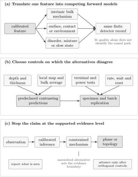
A feature first generates an alternative ledger, not a preferred label. Controls should make the alternatives predict different outcomes: depth and thickness test surface–bulk assignments; mapping and replication test inhomogeneity; terminal permutations test contacts; rate and waiting-time tests probe memory. The resulting claim stops at the highest evidence level supported by all checks.

The audit can be applied before data collection:

1. Define the feature numerically. Specify the fit, threshold, symmetry, localization, or scaling rule without naming a mechanism.
2. Write an alternative ledger. Include at least the proposed intrinsic mechanism, one specimen or disorder explanation, and one apparatus or analysis explanation.
3. Draw the forward paths. List which material variables, nuisance variables, and processing operations connect each alternative to the record.
4. Rank discriminating controls. Prefer controls that make leading alternatives predict different signs, scalings, locations, timescales, or null results.
5. Set acceptance criteria. Decide what result would support, weaken, or falsify each model before inspecting the control data.
6. Replicate at the right level. Repeat records for precision, cooldowns for stability, specimens for material claims, and batches or laboratories for generality.
7. Stop the claim at the evidence boundary. Report unresolved alternatives and the next decisive test.

One convenient alternative ledger is:

Candidate explanation	Distinctive prediction	Main nuisance	Discriminating control	Current status
Intrinsic bulk mechanism	Volume scaling and agreement among bulk probes	calibration and model parameters	thickness series plus thermodynamics	supported, weakened, or open
Surface or interface state	depth, termination, or gate dependence	aging and reconstruction	depth-sensitive spectroscopy	supported, weakened, or open
Inhomogeneous mixture	spatial variation and phase-fraction scaling	probe kernel	local map plus bulk average	supported, weakened, or open
Contact or heating artifact	terminal, power, or duty-cycle dependence	geometry and thermal path	permutations and low-power limit	supported, weakened, or open
Nonequilibrium memory	rate, wait-time, and reset dependence	controller lag	stabilized steps and reversal protocol	supported, weakened, or open

The ledger should evolve with the experiment. An alternative removed by one test can return if a later fabrication change invalidates that test.

Common Mistakes

• Describing a correlation with causal verbs before an intervention or discriminating prediction.
• Comparing one favored model only with a featureless background.
• Treating a low residual or high coefficient of determination as proof of microscopic correctness.
• Counting repeat scans as independent sample replication.
• Reporting only selected devices, cleaves, spatial regions, or fit windows.
• Averaging surface and bulk probes without their depth kernels and normalizations.
• Applying a linear phase-fraction mixture to transport near percolation.
• Assuming four-terminal sensing eliminates contact invasiveness, current jetting, and heating.
• Inferring a bulk phase from a percolating low-resistance path.
• Calling one edge state, band inversion, negative magnetoresistance, plateau, or zero-bias peak a topological invariant.
• Averaging hysteresis branches before testing whether they are distinct states.
• Assigning physical meaning to loop area without conjugate variables and units.
• Quoting statistical uncertainty while omitting calibration, model discrepancy, sample variation, and selection.
• Using post hoc exclusions without showing how the conclusion changes when they are restored.
• Treating failure of one alternative model as proof of the preferred model.

Exercises

1. Separate surface and bulk conductance

Two flakes of the same material have thicknesses $t_1=20\,\mathrm{nm}$ and $t_2=80\,\mathrm{nm}$. Their measured sheet conductances are $G_{\square,1}=1.8\,\mathrm{mS}$ and $G_{\square,2}=3.6\,\mathrm{mS}$. Assume

$$G_{\square}(t) = 2G_{\mathrm s} + \sigma_{\mathrm b}t,$$

with identical top and bottom surface conductances $G_{\mathrm s}$. Find $\sigma_{\mathrm b}$ and $G_{\mathrm s}$. Predict $G_{\square}$ for $t=50\,\mathrm{nm}$. State one reason the result would not prove topological surface transport.

Solution

The slope gives

$$\begin{aligned} \sigma_{\mathrm b} &= \frac{ 3.6-1.8 }{ 80-20 } \frac{\mathrm{mS}}{\mathrm{nm}} \\ &= 0.030\, \frac{\mathrm{mS}}{\mathrm{nm}} = 3.0\times10^4\,\mathrm{S\,m^{-1}}. \end{aligned}$$

The zero-thickness intercept is

$$\begin{aligned} 2G_{\mathrm s} &= 1.8\,\mathrm{mS} - \left( 0.030\, \frac{\mathrm{mS}}{\mathrm{nm}} \right) (20\,\mathrm{nm}) \\ &= 1.2\,\mathrm{mS}, \end{aligned}$$

so each surface contributes $G_{\mathrm s}=0.60\,\mathrm{mS}$. At $50\,\mathrm{nm}$,

$$G_{\square} = 1.2\,\mathrm{mS} + (0.030\,\mathrm{mS\,nm^{-1}})(50\,\mathrm{nm}) = 2.7\,\mathrm{mS}.$$

The intercept is only evidence for a thickness-independent parallel channel under the model. Trivial accumulation layers, damaged surfaces, edge paths, or thickness-dependent bulk mobility are alternatives.

2. Compare two information depths

A reconstructed surface layer is $d=1.0\,\mathrm{nm}$ thick. For normalized exponential depth weighting, compute the surface fraction for $\lambda_1=0.60\,\mathrm{nm}$ and $\lambda_2=3.0\,\mathrm{nm}$. Why does comparing the two settings help?

Solution

Using $f_{\mathrm{surf}}=1-e^{-d/\lambda}$,

$$\begin{aligned} f_{\mathrm{surf},1} &= 1-e^{-1/0.60} \simeq 0.811, \\ f_{\mathrm{surf},2} &= 1-e^{-1/3} \simeq 0.283. \end{aligned}$$

The first setting is dominated by the reconstructed layer, while the second gives much greater relative weight to deeper material. A feature that scales with these fractions supports a near-surface assignment. The test remains model dependent because matrix elements, elastic scattering, and the depth profile may also change between settings.

3. Show why phase fractions do not determine transport

A composite contains fraction $f=0.20$ of phase $A$ with $\sigma_A=1000\,\mathrm{S\,m^{-1}}$ and fraction $1-f$ of phase $B$ with $\sigma_B=10\,\mathrm{S\,m^{-1}}$. Compute the effective conductivity for ideal parallel stripes and ideal series layers.

Solution

For stripes parallel to current,

$$\begin{aligned} \sigma_{\parallel} &= f\sigma_A+(1-f)\sigma_B \\ &= 0.20(1000)+0.80(10) \\ &= 208\,\mathrm{S\,m^{-1}}. \end{aligned}$$

For layers in series,

$$\begin{aligned} \frac{1}{\sigma_{\mathrm{series}}} &= \frac{f}{\sigma_A} + \frac{1-f}{\sigma_B}, \\ \sigma_{\mathrm{series}} &= \left( \frac{0.20}{1000} + \frac{0.80}{10} \right)^{-1} \\ &\simeq 12.47\,\mathrm{S\,m^{-1}}. \end{aligned}$$

The same fractions and local conductivities differ by more than an order of magnitude because connectivity differs. A phase fraction from diffraction cannot be converted into transport without a geometry or network model.

4. Audit a contact-dependent magnetoresistance

At high field, two nominally longitudinal voltage pairs on the same anisotropic crystal give resistance changes of $-65\%$ and $+18\%$ under the same current contacts. Exchanging the current contacts changes the first result to $-12\%$. What can be concluded, and what should be done next?

Solution

The experiment has established strongly configuration-dependent terminal resistances. It has not established a unique intrinsic longitudinal resistivity. The sign and magnitude changes are evidence that current distribution, contact geometry, tensor mixing, or inhomogeneity matter.

Next steps include mapping all available terminal configurations, imaging the exact geometry, measuring field-angle and current dependence, checking reciprocity in the linear regime, and solving the anisotropic potential problem with measured contacts and dimensions. A chiral-anomaly interpretation should remain at most a candidate until current jetting and other magnetoresistance mechanisms are quantitatively bounded.

5. Derive a sweep-rate lag

Let $x_{\mathrm{eq}}(\lambda)=a\lambda$ and $\dot{\lambda}=r$. In the slow-ramp limit of

$$\dot{x} = - \frac{x-x_{\mathrm{eq}}}{\tau},$$

find the lag from equilibrium and the separation between equal-magnitude upward and downward ramps at the same $\lambda$.

Solution

The leading slow-ramp solution is

$$x \simeq x_{\mathrm{eq}} - \tau r \frac{dx_{\mathrm{eq}}}{d\lambda} = a\lambda-a\tau r.$$

Thus the lag is

$$\delta x = x-x_{\mathrm{eq}} = -a\tau r.$$

For upward and downward ramps with rates $+|r|$ and $-|r|$,

$$x_{\uparrow}-x_{\downarrow} = -2a\tau |r|.$$

The magnitude of the branch separation is $2|a|\tau|r|$ and vanishes linearly with sweep rate in this approximation. A rate-dependent loop therefore need not imply an equilibrium first-order transition.

6. Interpret an information-criterion comparison

Model $A$ has $k_A=3$ fitted parameters and $\ln\widehat{\mathcal L}_A=-120$. Model $B$ has $k_B=6$ and $\ln\widehat{\mathcal L}_B=-116$. Compute both AIC values. Is either mechanism proved?

Solution

The values are

$$\begin{aligned} \mathrm{AIC}_A &= 2(3)-2(-120) = 246, \\ \mathrm{AIC}_B &= 2(6)-2(-116) = 244. \end{aligned}$$

Model $B$ has the lower AIC by $2$, so it has modest support relative to $A$ within this candidate set and likelihood model. Neither mechanism is proved. The comparison does not include unconsidered alternatives, validate the noise model, establish causal direction, or test prediction outside the fitted data. Residual structure and held-out measurements could reverse the practical preference.

7. Calibrate a topological claim

A nanowire device shows a zero-bias conductance peak over a finite field interval. The peak appears only at one end, the induced gap softens with field, and no bulk-gap closing or reopening is resolved. Write the strongest justified claim and propose three discriminating tests.

Solution

The strongest justified statement is: the device has a local zero-bias feature compatible with several subgap mechanisms. The data do not establish a bulk topological phase or a nonlocal Majorana mode. Ordinary Andreev bound states, a quantum dot, disorder, dissipation, and heating remain viable.

Discriminating tests include:

1. simultaneous spectroscopy from both ends and a middle or bulk-sensitive terminal;
2. calibrated tracking of the induced bulk gap through the proposed transition, including field-angle and gate dependence;
3. replication across device length, barrier settings, contacts, and independently characterized disorder.

A later fusion or braid-order protocol would test non-Abelian operation at a still higher evidence level. It cannot be inferred from the local peak alone.

Research Status

• Established: forward-model comparison, uncertainty budgets, depth weighting, hierarchical replication, current-distribution effects, percolation, finite-rate relaxation, and phase-specific topological invariants are standard parts of experimental reasoning.
• Context dependent: the appropriate nuisance model, effective information depth, sample population, mixture law, equilibrium timescale, and decisive control depend on the material and apparatus.
• Active: robust inference from multimodal materials data, spatially heterogeneous phases, automated model discovery, nonequilibrium state identification, and consensus experimental protocols for candidate topological platforms.
• Not established by one suggestive feature: a unique microscopic mechanism, a homogeneous bulk phase, a topological invariant, equilibrium, or protection against perturbations.

Connections

• How Quantum Matter Is Measured supplies the forward measurement chain and probe-coordinate ledger assumed here.
• Device Fabrication Concepts tracks contacts, gates, process disorder, packaging, and batch provenance before interpretation begins.
• Transport Measurements and Hall Measurements own terminal reductions, reversal protocols, tensor inversion, and transport-specific failure modes.
• Angle-Resolved Photoemission Spectroscopy and Scanning Tunneling Microscopy and Spectroscopy develop the surface-sensitive spectral inferences summarized here.
• Heat Capacity and Thermodynamics and Magnetic Susceptibility provide bulk-integrated checks with their own addenda, geometry, and equilibration cautions.
• Disorder in Quantum Matter defines random ensembles and distinguishes quantum, transport, and dephasing times.
• Competing Orders develops homogeneous coexistence, exclusion, and phase separation as distinct physical hypotheses.
• Topology in Quantum Matter gives the bulk-gap, symmetry, invariant, and evidence framework behind the topological claim ladder.
• Open Quantum Materials separates unconditional open-system dynamics, conditional evolution, response poles, and non-Hermitian effective models.
• Error Estimates treats numerical conditioning, bias, variance, and model error.
• Validation Tests gives the analogous verification contract for computational results.

References

1. Joint Committee for Guides in Metrology, Evaluation of Measurement Data: Guide to the Expression of Uncertainty in Measurement, JCGM 100:2008.
2. Joint Committee for Guides in Metrology, International Vocabulary of Metrology: Basic and General Concepts and Associated Terms, 3rd ed., JCGM 200:2012.
3. G. E. P. Box, “Science and Statistics”, Journal of the American Statistical Association 71, 791–799 (1976).
4. J. R. Platt, “Strong Inference”, Science 146, 347–353 (1964).
5. H. Akaike, “A New Look at the Statistical Model Identification”, IEEE Transactions on Automatic Control 19, 716–723 (1974).
6. J. Pearl, Causality: Models, Reasoning, and Inference, 2nd ed., Cambridge University Press (2009).
7. M. A. Hernán and J. M. Robins, Causal Inference: What If, Chapman & Hall/CRC (2020; continuously corrected online edition).
8. R. A. Fisher, The Design of Experiments, Oliver and Boyd (1935).
9. D. C. Montgomery, Design and Analysis of Experiments, 10th ed., Wiley (2019).
10. S. Kirkpatrick, “Percolation and Conduction”, Reviews of Modern Physics 45, 574–588 (1973).
11. Y. Imry and M. Wortis, “Influence of Quenched Impurities on First-Order Phase Transitions”, Physical Review B 19, 3580–3585 (1979).
12. M. P. Seah and W. A. Dench, “Quantitative Electron Spectroscopy of Surfaces: A Standard Data Base for Electron Inelastic Mean Free Paths in Solids”, Surface and Interface Analysis 1, 2–11 (1979).
13. C. J. Powell and A. Jablonski, “Surface Sensitivity of X-Ray Photoelectron Spectroscopy”, Nuclear Instruments and Methods in Physics Research A 601, 54–65 (2009).
14. R. D. dos Reis et al., “On the Search for the Chiral Anomaly in Weyl Semimetals: The Negative Longitudinal Magnetoresistance”, New Journal of Physics 18, 085006 (2016).
15. F. Arnold et al., “Negative Magnetoresistance without Well-Defined Chirality in the Weyl Semimetal TaP”, Nature Communications 7, 11615 (2016).
16. M. Z. Hasan and C. L. Kane, “Colloquium: Topological Insulators”, Reviews of Modern Physics 82, 3045–3067 (2010).
17. N. P. Armitage, E. J. Mele, and A. Vishwanath, “Weyl and Dirac Semimetals in Three-Dimensional Solids”, Reviews of Modern Physics 90, 015001 (2018).
18. H. Pan and S. Das Sarma, “Physical Mechanisms for Zero-Bias Conductance Peaks in Majorana Nanowires”, Physical Review Research 2, 013377 (2020).
19. E. Prada et al., “From Andreev to Majorana Bound States in Hybrid Superconductor–Semiconductor Nanowires”, Nature Reviews Physics 2, 575–594 (2020).
20. J. P. Sethna et al., “Hysteresis and Hierarchies: Dynamics of Disorder-Driven First-Order Phase Transformations”, Physical Review Letters 70, 3347–3350 (1993).

Summary

• An observed correlation supports a mechanism only after plausible causal alternatives make and survive different predictions.
• Surface and bulk probes measure differently weighted responses; depth, thickness, and extensive-scaling controls are needed to reconcile them.
• Repeat scans, cooldowns, specimens, and batches answer different reproducibility questions.
• Inhomogeneous phase fractions do not determine transport without connectivity and probe-weighting models.
• Four-terminal sensing does not remove current jetting, contact-induced modification, or heating.
• A topological claim links symmetry, bulk structure, invariant-compatible modeling, boundary or response evidence, and alternative controls.
• Hysteresis establishes history dependence; sweep-rate, waiting-time, reset, and thermometry tests are needed to identify its origin.