Bulk–Boundary Correspondence

Bulk–boundary correspondence is the equality between a topological mismatch in gapped bulk phases and a stable index carried by their interface. In a two-dimensional Chern insulator, the difference of bulk Chern numbers equals the net oriented spectral flow of interface modes. In a time-reversal-invariant topological insulator, a relative $\mathbb Z_2$ index fixes the parity rather than the signed number of boundary crossings. In interacting phases, the same obstruction may be matched by gapless modes, symmetry breaking, boundary degeneracy, or intrinsic boundary topological order.

This is stronger and subtler than the slogan “nontrivial bulk implies an edge state.” The correspondence:

• compares two bulks, even when one is called the vacuum;
• constrains a stable aggregate such as net chirality, crossing parity, or anomaly;
• allows termination-dependent trivial bands and removable counterpropagating pairs;
• requires a bulk spectral gap, mobility gap, or an explicitly stated gapless-slice construction;
• depends on the symmetry and locality assumptions used to define the phase;
• does not identify every in-gap boundary eigenstate as topological.

This page owns the general index statement, oriented edge-state counting, domain-wall derivation, interacting qualifications, and numerical strip checks. Chern Numbers in Band Theory owns bulk-projector formulas and gauge-invariant Chern-number algorithms. Edge and Surface States owns boundary phenomenology, scattering, finite-size effects, and experimental probes. Phase-specific invariants and evidence remain in Integer Quantum Hall Effect, Topological Insulators, Topological Superconductors, and Topological Order.

Required background. Topology in Quantum Matter supplies the relative phase-equivalence, protection, and evidence logic used by every branch below.

Helpful background. Chern Numbers in Band Theory supplies projector invariants, Edge and Surface States supplies boundary phenomenology, and Tight-Binding Models supplies the strip and domain-wall constructions used in explicit checks.

Scope and Convention Ledger

Consider an interface normal to $x$, with a left bulk at $x<0$ and a right bulk at $x>0$. Translation symmetry along $y$ makes $k_\parallel=k_y$ a good quantum number in the clean problem. Put the reference energy $E_F$ inside a common bulk gap and define

$$\Delta C = C_L-C_R.$$

A boundary branch crossing $E_F$ with positive group velocity

$$v_\parallel = \frac{1}{\hbar} \frac{\partial E}{\partial k_\parallel}$$

is counted as right-moving. With the interface orientation fixed in this way,

$$\chi_{\mathrm{edge}} = N_{\mathrm R}-N_{\mathrm L}.$$

Reversing the interface normal or the definition of positive $k_\parallel$ reverses both sign conventions. A claimed sign is meaningless unless the coordinate orientation, occupied-band convention, and charge convention are also stated.

Item	Convention used here	Qualification
bulk invariant	invariant of occupied states below $E_F$	it must be defined on both sides
interface mismatch	left minus right	vacuum is a chosen trivial reference
edge count	positive-slope minus negative-slope crossings	count only in a common projected bulk gap
finite strip	localize each state to a specified edge	the two physical edges have opposite orientations
symmetry-protected phase	preserve the defining symmetry at the boundary	breaking it changes the boundary constraint
interactions	use a many-body invariant or anomaly	single-particle poles need not survive
disorder	replace a spectral gap by a justified mobility gap when appropriate	crystal momentum and band crossings may disappear

The word bulk means the thermodynamic interior. The word boundary includes an edge of a two-dimensional sample, a surface of a three-dimensional sample, and an interface between two phases. An atomically sharp termination is not required: a smooth region in which Hamiltonian parameters interpolate between phases is an interface too.

The clean free-fermion theorem assumes a local Hermitian Hamiltonian and a bulk gap at the reference energy. Symmetry-protected versions additionally require the relevant on-site or crystalline symmetry. Stable equivalence permits adding decoupled trivial bands and local boundary orbitals. Those additions can change the visible spectrum without changing the boundary index.

Statement in Band Topology

Let

$$H_{\mathrm{bulk}}(\mathbf k)$$

be a periodic, gapped Bloch Hamiltonian, and let

$$P(\mathbf k) = \Theta\!\left(E_F-H_{\mathrm{bulk}}(\mathbf k)\right)$$

be its occupied projector. Opening the system normal to $x$ replaces $k_x$ by a real-space coordinate while retaining $k_\parallel$:

$$H_{\mathrm{bulk}}(k_x,k_\parallel) \longrightarrow \widehat H(k_\parallel).$$

The spectrum of $\widehat H(k_\parallel)$ contains projected bulk continua and may contain states localized near the interface. The bulk–boundary theorem does not usually pair each bulk eigenvector with one boundary eigenvector. It identifies two indices:

$$\partial[\nu_{\mathrm{bulk}}] = [\nu_{\mathrm{boundary}}],$$

where $\partial$ is the boundary map appropriate to the symmetry class. This abstract form is useful because Chern numbers, winding numbers, real $\mathbb Z_2$ indices, and superconducting indices do not all count the same kind of boundary object.

Chern insulators

For two-dimensional class-A insulators, the boundary index is the spectral flow through $E_F$. If every crossing is made transverse by an arbitrarily small generic perturbation, define

$$\operatorname{sf}_{E_F}\widehat H = \sum_{a} \operatorname{sgn} \left. \left( \frac{\partial E_a}{\partial k_\parallel} \right) \right|_{E_a=E_F}.$$

The bulk–boundary correspondence is

$$\operatorname{sf}_{E_F}\widehat H = N_{\mathrm R}-N_{\mathrm L} = C_L-C_R.$$

The equality is stable under local changes of boundary potential, hopping, reconstruction, and disorder that preserve the hypotheses. A termination can create three right-moving and two left-moving branches in the gap even when $\Delta C=1$. The two removable counterpropagating pairs are not separately protected; the difference is.

This is a relative theorem. Calling the right side “vacuum” means assigning it a trivial lattice regularization with $C_R=0$. Depositing an ordinary two-dimensional layer on a three-dimensional surface or adding boundary orbitals can alter the surface spectrum and even add an integer Hall layer. The physically stable statement compares fully specified adjoining phases.

One-dimensional chiral systems

For a one-dimensional Hamiltonian with chiral symmetry, a bulk winding mismatch gives a boundary zero-mode index. In a basis where the chiral operator is diagonal,

$$H(k) = \begin{pmatrix} 0 & q(k)\\ q^\dagger(k) & 0 \end{pmatrix},$$

the winding of $\det q(k)$ is

$$\nu = \frac{1}{2\pi i} \int_{\mathrm{BZ}} dk\, \partial_k\log\det q(k).$$

At an interface, the difference $\nu_L-\nu_R$ fixes a signed sublattice zero-mode count. The SSH Model is the canonical elementary realization. Its visible end state depends on termination because changing the cut changes which bulk and vacuum conventions are being compared. Chiral-symmetry-breaking boundary terms can shift a zero mode away from zero even when a boundary-localized state remains.

Kramers crossing parity in time-reversal-invariant insulators

For a two-dimensional class-AII topological insulator, time reversal forces the total charge Chern number to vanish. The stable boundary datum is instead a parity:

$$\mathcal P_{\mathrm{edge}} = \nu_L\oplus\nu_R \in \mathbb Z_2.$$

An odd mismatch requires odd partner switching between boundary time-reversal-invariant momenta. Boundary reconstruction may add two Kramers pairs and change three visible crossings into five, but it cannot change odd to even without closing the bulk gap, breaking time reversal, or coupling to another anomalous boundary.

For a three-dimensional strong topological insulator, an odd surface Dirac-cone parity is the free-fermion signature on a symmetry-preserving surface. Weak indices are orientation-sensitive: a surface that breaks the protecting translation structure or projects weak layers in an unfavorable direction need not display the same robust cones. Crystalline phases similarly require a boundary that preserves the relevant mirror, rotation, glide, or other spatial symmetry.

Superconductors and neutral modes

Bogoliubov–de Gennes Hamiltonians have particle–hole redundancy rather than ordinary charge conservation. Their boundary index can enforce Majorana zero modes, chiral Majorana spectral flow, or helical Majorana cones. Counting complex electronic channels would double-count the degrees of freedom. Topological Superconductors owns the phase-specific invariants and fermion-parity constraints.

Gapless bulk slices

A Weyl semimetal has no three-dimensional bulk gap at the nodes, so the gapped-insulator theorem cannot be applied to the entire Brillouin zone. Instead, two-dimensional momentum slices between Weyl nodes can carry nonzero Chern number. Their edge states assemble into a surface Fermi arc. As a slice approaches a node, its gap closes and the boundary state merges into the projected bulk continuum. Weyl and Dirac Semimetals owns this slice construction and the projection caveats.

The main free-fermion cases can therefore be summarized without pretending that every invariant is an integer channel count:

Bulk datum	Boundary datum	Stable operation
Chern-number difference $\Delta C$	net chiral spectral flow	add or remove counterpropagating pairs
chiral winding difference $\Delta\nu$	signed zero-mode index	add trivial boundary dimers
class-AII $\mathbb Z_2$ mismatch	Kramers-pair crossing parity	add two Kramers pairs
strong three-dimensional $\mathbb Z_2$ mismatch	odd surface-cone anomaly	add an even number of cones
BdG integer or parity invariant	Majorana channel or zero-mode index	add topologically trivial BdG bands
Weyl-slice Chern number	arc segment in that gapped slice	deform the arc while endpoints remain tied to projected nodes

Spectral Flow, Pumping, and Anomaly

The same correspondence has several complementary formulations. They agree on the stable index but expose different physics.

Flux insertion as a counting argument

Put a Chern insulator on a cylinder and thread flux $\Phi$ through its hole. A flux quantum

$$\Phi_0 = \frac{h}{e}$$

returns the Hamiltonian to a gauge-equivalent form. The adiabatic cycle shifts the allowed momentum around the circumference by one spacing. For a filled Chern band, the charge pumped from one boundary to the other is

$$\Delta Q = C e.$$

If the bulk remains gapped throughout the cycle, this charge cannot be supplied by a bulk level crossing at $E_F$. Boundary occupation must change. The net number of boundary levels crossing the reference energy is therefore $C$, with opposite signs on the two ends of the cylinder. This is the spectral-flow form of the Laughlin pump. The phase-specific Hall-bar and reservoir treatment remains in Integer Quantum Hall Effect.

Berry-Phase Polarization and Charge Pumping owns the distinct one-dimensional crystalline-pump ledger: continuous polarization branches, ionic-plus-electronic charge, the $(k,t)$ torus, and the integrated bulk current. This page retains the boundary spectral-flow and relative-index statement.

This argument also explains why counting both boundaries of a finite strip without localization labels gives zero net chirality. Charge leaving one boundary arrives at the other. Each boundary separately carries the index appropriate to its outward orientation.

Chern–Simons response and anomaly inflow

At long wavelength, a two-dimensional Chern phase has the electromagnetic response

$$S_{\mathrm{bulk}}[A] = \frac{C e^2}{4\pi\hbar} \int_M A\wedge dA.$$

On a closed spacetime, the action is gauge invariant up to the usual quantization conditions. When $M$ has a boundary, a gauge transformation $A\mapsto A+d\lambda$ produces a boundary term:

$$\delta_\lambda S_{\mathrm{bulk}} = \frac{C e^2}{4\pi\hbar} \int_{\partial M} \lambda\,dA,$$

up to the sign fixed by boundary orientation. A purely one-dimensional chiral theory has the complementary gauge anomaly. The combined bulk-plus-boundary system is gauge consistent: charge apparently lost by the boundary is supplied by Hall inflow from the bulk.

Anomaly inflow is more general than a free edge-band plot. It remains meaningful when interactions destroy a quasiparticle description, provided the symmetry and response assumptions are stated. It also clarifies why an anomalous boundary cannot be realized as an isolated lower-dimensional, symmetry-preserving, short-range-entangled system.

Physical, Wannier, and entanglement spectra

Several spectra can exhibit related flow:

• a physical boundary spectrum is obtained by opening the Hamiltonian and can carry transport;
• a Wilson-loop or hybrid-Wannier spectrum is built from occupied bulk states and diagnoses their geometry;
• an entanglement spectrum is built from a reduced density operator or correlation matrix across a virtual cut.

Their resemblance can be powerful, but they are not interchangeable measurements. A Wilson-loop crossing does not by itself provide a conducting channel. An entanglement level is not a physical excitation energy. Entanglement Spectrum owns the virtual-boundary construction and its interacting qualifications.

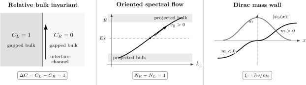
Three compatible views of the same stable obstruction. A relative invariant $\Delta C$ fixes oriented spectral flow through a common bulk gap. In a continuum Dirac representative, a sign-changing mass localizes the corresponding channel, but the integer claim belongs to the complete lattice-regulated bulk.

Edge-State Counting

Count oriented crossings, not visible branches

Choose $E_F$ inside the projected bulk gap for every $k_\parallel$ used in the count. For each boundary-localized branch, record every transverse crossing and its velocity sign. A branch that enters the gap, turns around, and exits through the same bulk band contributes zero net spectral flow because its upward and downward crossings cancel.

At an accidental tangency,

$$\left. \frac{\partial E}{\partial k_\parallel} \right|_{E_F} = 0,$$

the sign is undefined. Shift $E_F$ slightly within the gap or add an arbitrarily small generic boundary perturbation. A stable index cannot depend on resolving a nongeneric tangency.

Raw branch counts fail for three common reasons:

1. trivial Tamm or Shockley states can enter the gap;
2. boundary reconstruction can add a right-left pair;
3. two nearby branches can hybridize and reconnect without changing the bulk.

The net count survives all three operations.

Localize the two edges of a strip

A strip of width $L_x$ has two boundaries. Let $\psi_n(x;k_\parallel)$ be a normalized strip eigenstate and choose an edge window of $x_c$ sites. Define

$$\begin{aligned} w_{n,L}(k_\parallel) &= \sum_{x=1}^{x_c} \lVert\psi_n(x;k_\parallel)\rVert^2, \\ w_{n,R}(k_\parallel) &= \sum_{x=L_x-x_c+1}^{L_x} \lVert\psi_n(x;k_\parallel)\rVert^2. \end{aligned}$$

A state should be assigned to an edge only when its weight and position expectation support that assignment. Coloring every eigenvalue by $\langle x\rangle$ is useful, but a broad bulk state can have the same mean position as a localized edge state. Also inspect the variance

$$\operatorname{Var}_n(x) = \langle x^2\rangle_n-\langle x\rangle_n^2$$

or fit the real-space envelope.

For a wide strip, the two edges carry opposite group velocities at the same energy because their outward normals are opposite. The localization-resolved index is nonzero at each edge, while the unlabelled sum over the entire finite strip vanishes.

Finite-width hybridization

If the left and right boundary envelopes decay with length $\xi$, their overlap opens an avoided crossing of order

$$\Delta_{\mathrm{fs}}(L_x) \sim A e^{-L_x/\xi},$$

possibly with an oscillatory prefactor in multivalley systems. A small strip gap is therefore not automatically evidence that the bulk phase is trivial or that its protecting symmetry is broken. Repeat the calculation for several widths. Exponential closure supports boundary hybridization; saturation to a nonzero value indicates a genuine allowed mass, a bulk or numerical error, or a different boundary problem.

Track states by overlap

Sorting eigenvalues independently at adjacent momenta can swap labels at crossings and avoided crossings. A more reliable branch tracker maximizes

$$\left| \left\langle \psi_m(k_\parallel+\delta k) \middle| \psi_n(k_\parallel) \right\rangle \right|^2$$

within a relevant energy window. Near degeneracies, track the whole nearly degenerate subspace with singular values or projectors rather than forcing an arbitrary one-state correspondence.

The final topological count should not depend on the tracking convention. Tracking is a numerical aid for assigning velocity and localization, not a replacement for the bulk invariant.

Domain Walls and Mass Sign Changes

A Dirac mass kink is the local continuum mechanism behind many boundary modes. It is a representative proof, not a substitute for the lattice theorem.

Two-dimensional Dirac interface

Take

$$H(k_y) = -i\hbar v\,\sigma_x\partial_x + \hbar v k_y\sigma_y + m(x)\sigma_z,$$

with

$$\lim_{x\to-\infty}m(x)=-m_0, \qquad \lim_{x\to+\infty}m(x)=+m_0, \qquad m_0>0.$$

At $k_y=0$, the zero-energy equation is

$$\left( -i\hbar v\,\sigma_x\partial_x + m(x)\sigma_z \right) \psi_0(x) = 0.$$

Using $\sigma_x\sigma_z=-i\sigma_y$ gives

$$\partial_x\psi_0(x) = -\frac{m(x)}{\hbar v} \sigma_y\psi_0(x).$$

Choose $\sigma_y\chi_s=s\chi_s$, where $s=\pm1$. Then

$$\psi_s(x) = \mathcal N \exp\left[ -\frac{s}{\hbar v} \int_0^x m(x')\,dx' \right] \chi_s.$$

For the stated mass orientation, the integral tends to $+\infty$ in both spatial directions. Only $s=+1$ is normalizable. Projecting the remaining momentum term onto that state gives

$$E_{\mathrm{dw}}(k_y) = \hbar v k_y.$$

Reversing the mass profile selects $s=-1$ and reverses the propagation direction. A scalar potential can bend or shift the branch, but it cannot remove an unpaired chiral spectral flow while the two asymptotic bulks and their common gap remain intact.

For a smooth kink

$$m(x) = m_0\tanh\left(\frac{x}{\ell}\right),$$

the envelope is explicit:

$$\psi_0(x) \propto \left[ \operatorname{sech}\left(\frac{x}{\ell}\right) \right]^{m_0\ell/(\hbar v)} \chi_+.$$

Far from the wall,

$$\lVert\psi_0(x)\rVert \sim e^{-\lvert x\rvert/\xi}, \qquad \xi = \frac{\hbar v}{m_0}.$$

The boundary penetrates more deeply as the bulk gap scale $m_0$ decreases. At a topological phase transition, $\xi$ diverges and the distinction between boundary and bulk modes disappears.

The regulator warning

A single continuum Dirac cone contributes a half-integer-looking Chern–Simons term. That number is not, by itself, the Chern number of a strictly two-dimensional lattice band. The ultraviolet regulator and all lattice Dirac points complete the integer invariant. What the kink calculation safely establishes is:

• a sign reversal of one regulated Dirac mass changes its contribution by an integer;
• the interface binds the corresponding oriented low-energy branch;
• the total branch count must be checked against the full lattice invariant.

Ignoring the regulator leads to factor-of-two and sign errors, especially when several valleys or spin blocks are present.

Multiple flavors and allowed masses

For several Dirac species, write the mass as a matrix in flavor space. Modes of opposite chirality can acquire a boundary gap when an allowed perturbation couples them. Schematically,

$$H_{\mathrm{pair}}(k) = \hbar v k\,\tau_z + \mu\,\tau_x,$$

with spectrum

$$E_\pm(k) = \pm \sqrt{(\hbar v k)^2+\mu^2}.$$

The mass $\mu$ removes one right-left pair but leaves the net chirality unchanged. A symmetry may forbid $\tau_x$ and turn an otherwise removable pair into a symmetry-protected helical boundary. This is why the symmetry class belongs in every bulk–boundary statement.

A mass wall on a surface

A magnetic coating can gap a topological-insulator surface Dirac cone. If the exchange mass changes sign along a line on that surface, the same calculation predicts a one-dimensional chiral channel bound to the magnetic domain wall. Here the “two bulks” are two gapped surface regions with different Hall responses, while the three-dimensional bulk supplies the anomalous half-integer offset. The measurable line channel depends on magnetic texture, chemical potential, and unwanted parallel conduction, but its direction reverses with the mass orientation.

Interacting and Disordered Caveats

Bands are no longer the fundamental objects

Strong interactions can destroy sharp single-particle quasiparticles. A many-body phase may still have a quantized response, ground-state obstruction, symmetry anomaly, or topological order. Bulk–boundary correspondence then relates those many-body data to all consistent boundary realizations, not necessarily to poles of a one-electron Green function.

Green-function poles and zeros at a boundary

For an interacting Green function $G(\omega,\mathbf k)$, a topological formula can change through either a pole or a zero. At an interface, a bulk mismatch can therefore be reflected in boundary poles, boundary zeros, or more collective degrees of freedom. A Green-function zero is not an observable electron edge mode; it records vanishing single-particle propagation. This is one reason not to promote a free-band crossing count into a universal interacting theorem.

Interactions can also reduce a free-fermion classification. The standard examples include

$$\mathbb Z \longrightarrow \mathbb Z_8$$

for one-dimensional class BDI and

$$\mathbb Z \longrightarrow \mathbb Z_{16}$$

for three-dimensional class DIII under the relevant interacting equivalence. Symmetry-Protected Topological Phases owns these reductions and the stable many-body phase relation.

Interacting gapped surfaces and topological order

An anomalous boundary of a nontrivial symmetry-protected phase cannot be simultaneously:

1. symmetry preserving;
2. fully gapped;
3. nondegenerate and short-range entangled;
4. realizable as an isolated system in the same dimension with the same symmetry action.

It may instead be:

• gapless, as in the weakly interacting surface Dirac cone;
• symmetry breaking, with degenerate boundary sectors and domain walls;
• symmetry preserving but topologically ordered, possible for suitable higher-dimensional boundaries;
• coupled to another anomalous boundary, so that the combined anomaly cancels.

The third option is crucial. A symmetry-preserving gapped surface of a three-dimensional electronic topological insulator does not refute bulk–boundary correspondence if that surface carries intrinsic anyon order. It realizes the anomaly in a way unavailable to an ordinary isolated two-dimensional electron system.

Intrinsic topological order need not have a gapless edge

A nonchiral topologically ordered phase can admit a fully gapped boundary through anyon condensation. Different condensable sets can define inequivalent boundary types, and junctions between them can bind protected defects. Thus “topological order implies a conducting edge” is false.

Chiral topological order is different. A nonzero chiral central charge produces a gravitational anomaly and thermal Hall response that obstruct a completely trivial gapped boundary to vacuum. The precise boundary classification depends on the anyon theory, condensable algebra, conserved symmetries, and whether extra invertible layers are allowed. Topological Order owns modular data, $K$ matrices, chiral response, and anyon-condensation caveats.

Disorder removes momentum, not the correspondence

With strong disorder, $k_\parallel$ and a clean edge dispersion may not exist. In an integer quantum Hall phase, a mobility gap and noncommutative Chern number can still define the bulk invariant. The boundary statement becomes quantized edge current, robust transport, or the impossibility of localizing all boundary degrees of freedom under the theorem’s hypotheses, rather than a literal band crossing on an $E$–$k$ plot.

Numerically, disorder should be tested with:

• twisted boundary conditions or a real-space Chern/Bott index;
• localization diagnostics and system-size scaling;
• boundary current or scattering observables;
• disorder averaging with uncertainty estimates;
• a check that the Fermi energy lies in a mobility gap rather than merely a low finite-size density of states.

Long-range interactions, non-Hermitian effective generators, Floquet drives, and open-system steady states require modified correspondences. Their invariants and boundary spectra should not be inferred by importing the static local Hermitian theorem unchanged.

A Lattice-Regulated Example

Consider the two-band Qi–Wu–Zhang Hamiltonian

$$H(\mathbf k) = \sin k_x\,\sigma_x + \sin k_y\,\sigma_y + \left( M+\cos k_x+\cos k_y \right)\sigma_z.$$

The lattice spacing and hopping scale are set to one. The gap can close only where $\sin k_x=\sin k_y=0$, at the four high-symmetry momenta. Their masses and Dirac chiralities are

Momentum	Mass	Chirality
$\Gamma=(0,0)$	$M+2$	$+1$
$X=(\pi,0)$	$M$	$-1$
$Y=(0,\pi)$	$M$	$-1$
$M_{\mathrm{BZ}}=(\pi,\pi)$	$M-2$	$+1$

For the lower band and the orientation used here,

$$C = -\frac{1}{2} \left[ \operatorname{sgn}(M+2) -2\operatorname{sgn}(M) +\operatorname{sgn}(M-2) \right].$$

Hence

$$C = \begin{cases} 0, & M<-2,\\ -1, & -2<M<0,\\ +1, & 0<M<2,\\ 0, & M>2. \end{cases}$$

The invariant is undefined at $M=-2,0,2$, where the bulk gap closes. Different Pauli-matrix, band, or Brillouin-zone orientations can reverse every displayed Chern sign without changing the physical correspondence.

Open strip Hamiltonian

Open the $x$ direction and retain $k_y$. Use the Fourier convention

$$c_x = \frac{1}{\sqrt{L_x}} \sum_{k_x} e^{-ik_xx} c_{k_x}.$$

Then write

$$h_0(k_y) = \sin k_y\,\sigma_y + \left(M+\cos k_y\right)\sigma_z$$

and

$$T = \frac{1}{2} \left( \sigma_z-i\sigma_x \right).$$

The strip Hamiltonian with $L_x$ cells is

$$\begin{aligned} H_{\mathrm{strip}}(k_y) &= \sum_{x=1}^{L_x} c_x^\dagger h_0(k_y)c_x \\ &\quad+ \sum_{x=1}^{L_x-1} \left( c_{x+1}^\dagger T c_x + c_x^\dagger T^\dagger c_{x+1} \right). \end{aligned}$$

With the opposite Fourier phase, $T$ and $T^\dagger$ exchange places. In either convention, reconstruct the periodic Hamiltonian before interpreting any Chern sign.

For $M=1$, the bulk lower band has $C=+1$. A wide strip contains one oriented crossing at each edge, with opposite slopes because the edges have opposite normals. For $M=3$, $C=0$ and no net crossing is required, although a special boundary potential may still produce topologically trivial in-gap states.

Numerical Workflow and Checks

A convincing numerical demonstration compares independent bulk and boundary calculations.

1. Verify the bulk problem

1. Diagonalize the periodic Hamiltonian on a converged momentum mesh.
2. Confirm a nonzero direct gap everywhere and the intended filling.
3. Compute the occupied-band Chern number with a gauge-invariant plaquette method.
4. Refine the mesh until the integer and minimum gap are stable.
5. Check at least one analytically known parameter point.

The plaquette algorithm and its admissibility checks are canonical in Chern Numbers in Band Theory.

2. Build and validate the strip

Construct $H_{\mathrm{strip}}(k_y)$ and first verify that imposing periodic $x$ boundary conditions reproduces $H(k_x,k_y)$. Hermiticity alone does not catch a reversed hopping or Fourier sign.

For each $k_y$:

1. diagonalize in an energy window around the common bulk gap;
2. compute left and right edge weights;
3. track boundary subspaces by overlap;
4. locate crossings of a fixed $E_F$;
5. estimate slopes and assign signs;
6. report the count separately for each edge.

A practical crossing count should state the momentum spacing, interpolation method, energy tolerance, localization threshold, and treatment of degeneracies.

3. Converge width and boundary details

Repeat the strip calculation for several $L_x$. The bulk gap should remain fixed while a hybridization gap between opposite edges decays exponentially. Then change the boundary onsite energy or the first few hoppings. Individual branches may move or extra pairs may appear, but the localization-resolved net count must remain $\Delta C$.

4. Check spectral weight, not just eigenvalues

The boundary spectral function

$$A_{\mathrm{edge}}(k_\parallel,\omega) = -\frac{1}{\pi} \operatorname{Im} \operatorname{Tr} \left[ W_{\mathrm{edge}} G^R(k_\parallel,\omega) \right]$$

uses a projector $W_{\mathrm{edge}}$ onto an edge window. It distinguishes an edge-localized pole from a bulk eigenvalue plotted in the same energy range. With finite broadening $\eta$, repeat the plot for several $\eta$ values so numerical linewidth is not mistaken for a physical lifetime.

5. Use real-space diagnostics when translation is absent

For disorder or irregular boundaries, compare a real-space bulk index with boundary response. A local Chern marker can be written schematically as

$$\mathcal C(\mathbf r) = -4\pi \operatorname{Im} \left\langle\mathbf r\right| P X(1-P)Y P \left|\mathbf r\right\rangle,$$

with normalization adjusted to the lattice-cell convention. Deep in a large clean sample, its spatial average approaches the bulk Chern number. Near a boundary it is not locally quantized, and the trace over a finite sample must satisfy compensating sum rules. The Bott index provides another finite real-space diagnostic. Neither number excuses a missing finite-size or mobility-gap analysis.

Acceptance ledger

Check	Expected topological result	Common false positive
bulk invariant	stable integer or parity under refinement	premature rounding on a coarse mesh
bulk gap	nonzero at intended filling	checking only high-symmetry points
boundary localization	weight concentrated near one interface	coloring a delocalized state by mean position
oriented crossing count	equals the relative bulk invariant	counting all in-gap bands without velocity signs
strip-width scaling	hybridization gap closes as $e^{-L_x/\xi}$	declaring one narrow strip trivial
boundary perturbation	branches deform but stable index persists	treating one special termination as universal
disorder test	mobility gap and real-space index agree	low density of states mistaken for localization
independent method	bulk and boundary calculations concur	reusing the same flawed convention in both

Common Mistakes

Treating every boundary state as topological

Ordinary surface potentials, dangling bonds, and reconstruction can create in-gap states. The correspondence constrains a stable index, not the existence of any one branch.

Counting bands without orientation

Two counterpropagating branches contribute zero net chirality. Count signed crossings at a common reference energy.

Counting both strip edges together

The two edges have opposite orientations, so their unlabelled net spectral flow cancels. Use localization-resolved counts.

Ignoring the projected bulk gap

A boundary-looking state inside the global energy range may overlap the projected bulk continuum at the same $k_\parallel$. There it can hybridize with bulk states and is not an isolated edge branch.

Using one continuum cone as an integer lattice invariant

A continuum Dirac mass diagnoses a local transition and domain-wall mode. The complete lattice regulator determines the integer invariant.

Forgetting the protecting symmetry

A time-reversal-protected edge can be gapped by a time-reversal-breaking boundary perturbation without changing the bulk phase. The gapped boundary then carries the anomaly through its symmetry breaking and domain walls.

Equating gapless boundary with the only interacting option

A symmetry-preserving boundary can be gapped by intrinsic topological order, and a nonchiral topological order can have a gapped boundary through anyon condensation.

Reading a finite-size gap as a boundary mass

Opposite edges hybridize exponentially in a narrow strip. Width scaling separates this overlap from a genuine symmetry-allowed mass.

Claiming a disorder theorem from a clean band plot

When momentum is lost, use mobility-gap, real-space-index, localization, and transport diagnostics. A broadened clean dispersion is not a disordered bulk–boundary proof.

Exercises

1. Stable versus raw channel counts

An interface has $C_L=2$ and $C_R=-1$. A particular termination shows five right-moving and two left-moving crossings at $E_F$. Is the spectrum consistent with bulk–boundary correspondence? How many pairs can be removed without changing the bulk?

Solution

The relative invariant is

$$\Delta C = C_L-C_R = 2-(-1) = 3.$$

The boundary count is

$$N_{\mathrm R}-N_{\mathrm L} = 5-2 = 3,$$

so it is consistent. Two right-left pairs can be coupled and removed by generic boundary perturbations, leaving three unpaired right-moving branches. The correspondence fixes the net three, not the raw total of seven crossings.

2. Gap a removable pair

Consider two counterpropagating boundary modes described by

$$H_0(k) = \hbar v k\,\tau_z.$$

Show that a momentum-independent coupling $\mu\tau_x$ gaps the pair, and explain why this does not change a Chern boundary index.

Solution

The coupled Hamiltonian is

$$H(k) = \hbar v k\,\tau_z + \mu\tau_x.$$

Since $\{\tau_z,\tau_x\}=0$,

$$H^2 = (\hbar v k)^2+\mu^2,$$

and therefore

$$E_\pm(k) = \pm \sqrt{(\hbar v k)^2+\mu^2}.$$

The gap is $2\lvert\mu\rvert$. Before coupling, one branch has positive slope and one has negative slope, so their net chirality is zero. Removing them leaves $N_{\mathrm R}-N_{\mathrm L}$ unchanged. If a symmetry forbids $\tau_x$, the same pair may instead be symmetry protected.

3. Solve a smooth Dirac mass kink

For

$$m(x) = m_0\tanh(x/\ell),$$

derive the normalizable zero-mode envelope and its asymptotic penetration depth.

Solution

For the normalizable $\sigma_y=+1$ spinor,

$$\psi_0(x) = \mathcal N \exp\left[ -\frac{1}{\hbar v} \int_0^x m(x')\,dx' \right] \chi_+.$$

The integral is

$$\int_0^x m_0\tanh(x'/\ell)\,dx' = m_0\ell \log\cosh(x/\ell).$$

Hence

$$\psi_0(x) = \mathcal N \left[ \operatorname{sech}(x/\ell) \right]^{m_0\ell/(\hbar v)} \chi_+.$$

For $\lvert x\rvert\gg\ell$,

$$\operatorname{sech}(x/\ell) \sim 2e^{-\lvert x\rvert/\ell},$$

so

$$\lVert\psi_0(x)\rVert \sim e^{-m_0\lvert x\rvert/(\hbar v)}.$$

The penetration depth is

$$\xi = \frac{\hbar v}{m_0}.$$

4. Derive the lattice phase diagram

Use the four Dirac masses of the Qi–Wu–Zhang model to evaluate

$$C = -\frac{1}{2} \left[ \operatorname{sgn}(M+2) -2\operatorname{sgn}(M) +\operatorname{sgn}(M-2) \right]$$

in every gapped interval.

Solution

For $M>2$, all three sign arguments are positive:

$$C = -\frac12(1-2+1) = 0.$$

For $0<M<2$,

$$C = -\frac12(1-2-1) = +1.$$

For $-2<M<0$,

$$C = -\frac12(1+2-1) = -1.$$

For $M<-2$, all arguments are negative:

$$C = -\frac12(-1+2-1) = 0.$$

At $M=-2,0,2$, at least one Dirac mass vanishes, so the bulk is gapless and the occupied-band Chern number is not defined.

5. Diagnose a finite-strip gap

A strip calculation gives avoided-crossing gaps

$$\begin{array}{c|ccc} L_x & 20 & 30 & 40\\ \hline \Delta_{\mathrm{fs}} & 0.0733 & 0.0270 & 0.00993 \end{array}$$

in fixed energy units. Test whether the data are consistent with $\Delta_{\mathrm{fs}}\propto e^{-L_x/\xi}$ and estimate $\xi$.

Solution

For two widths separated by $\Delta L=10$,

$$\frac{\Delta_{\mathrm{fs}}(L)} {\Delta_{\mathrm{fs}}(L+10)} \approx e^{10/\xi}.$$

The first ratio is

$$\frac{0.0733}{0.0270} \approx 2.715,$$

and the second is

$$\frac{0.0270}{0.00993} \approx 2.719.$$

Both are close to $e$. Therefore

$$\frac{10}{\xi} \approx 1, \qquad \xi \approx 10$$

lattice spacings. The consistent exponential ratio supports opposite-edge hybridization. More widths and localization profiles should still be checked before excluding oscillatory or multi-length-scale corrections.

6. Crossing parity under edge reconstruction

Two time-reversal-preserving terminations of the same two-dimensional topological insulator show three and five Kramers-pair crossings, respectively, between the two boundary time-reversal-invariant momenta. Can both represent the same bulk phase?

Solution

Yes. The class-AII boundary invariant is the parity:

$$3\bmod2 = 5\bmod2 = 1.$$

Boundary reconstruction has added two Kramers-pair crossings, which is topologically trivial under stable equivalence. Either termination has odd partner switching and therefore matches the same nontrivial relative $\mathbb Z_2$ invariant. A change from odd to even would require breaking the assumptions or changing the bulk.

7. Classify interacting boundary outcomes

A three-dimensional electron topological insulator has three proposed time-reversal-symmetric surface states:

1. a gapless Dirac surface;
2. a fully gapped, nondegenerate, short-range-entangled surface with no anyons;
3. a fully gapped surface with intrinsic non-Abelian topological order.

Which are compatible with bulk–boundary correspondence?

Solution

The gapless Dirac surface is compatible: its low-energy modes carry the anomaly.

The second proposal is incompatible if it truly preserves the full symmetry, is nondegenerate and short-range entangled, and is an isolated termination. It supplies no boundary mechanism for the nontrivial bulk anomaly.

The third proposal is compatible. Intrinsic surface topological order can preserve time reversal while realizing an anomalous symmetry action unavailable to a strictly two-dimensional short-range-entangled electron system. Gapping the single-particle spectrum therefore does not erase the correspondence.

8. Audit a numerical bulk–boundary claim

A calculation reports $C=-1$ on a $21\times21$ momentum mesh. A width-$24$ strip shows a small gap and no exact crossing, so the authors conclude that bulk–boundary correspondence fails. List the minimum checks needed before accepting that conclusion.

Solution

At minimum:

1. refine the momentum mesh and report the minimum direct bulk gap;
2. verify the intended occupied-band filling and Chern-sign convention;
3. reconstruct the periodic Bloch Hamiltonian from the strip hopping matrices;
4. compute edge weights rather than inspecting eigenvalues alone;
5. repeat for several strip widths and test exponential gap closure;
6. vary boundary onsite terms to distinguish stable flow from a special termination;
7. track near-degenerate boundary subspaces by overlap;
8. count oriented crossings at a reference energy inside the projected bulk gap.

If the strip gap decays as $e^{-L_x/\xi}$, the width-$24$ result is finite-size hybridization and is consistent with the correspondence. A persistent gap would still require checking whether a protecting symmetry was broken, whether the two compared bulks were specified correctly, and whether the numerical Hamiltonian implements the claimed model.

Connections

• Topology in Quantum Matter supplies the phase-equivalence, invariant, response, and evidence overview.
• Chern Numbers in Band Theory owns occupied-projector geometry, lattice regularization, Hall response, and gauge-invariant bulk algorithms.
• Edge and Surface States develops chiral, helical, Dirac, Majorana, and Fermi-arc phenomenology with experimental probes.
• Integer Quantum Hall Effect develops chiral channels, flux insertion, mobility gaps, localization, and multi-terminal transport.
• Topological Insulators owns class-AII invariants, helical edges, strong and weak indices, and material evidence.
• Symmetry-Protected Topological Phases owns interacting phase equivalence, anomalous boundaries, and classification reductions.
• Topological Order owns anyon data, chiral central charge, gapped boundaries, and anyon-condensation qualifications.
• Entanglement Spectrum develops the virtual-boundary spectrum and its relation to physical edges.
• SSH Model is the compact one-dimensional chiral-symmetry model card.
• Green Functions in Many-Body QM provides the pole, zero, and spectral language needed for interacting qualifications.

Further Reading

• E. Prodan and H. Schulz-Baldes, Bulk and Boundary Invariants for Complex Topological Insulators: From K-Theory to Physics, Springer (2016), doi:10.1007/978-3-319-29351-6.
• G. M. Graf and M. Porta, “Bulk–Edge Correspondence for Two-Dimensional Topological Insulators,” Communications in Mathematical Physics 324, 851–895 (2013), doi:10.1007/s00220-013-1819-6.
• A. M. Essin and V. Gurarie, “Bulk–Boundary Correspondence of Topological Insulators from Their Respective Green’s Functions,” Physical Review B 84, 125132 (2011), doi:10.1103/PhysRevB.84.125132.
• C.-K. Chiu, J. C. Y. Teo, A. P. Schnyder, and S. Ryu, “Classification of Topological Quantum Matter with Symmetries,” Reviews of Modern Physics 88, 035005 (2016), doi:10.1103/RevModPhys.88.035005.

References

Bulk and edge indices

1. B. I. Halperin, “Quantized Hall Conductance, Current-Carrying Edge States, and the Existence of Extended States in a Two-Dimensional Disordered Potential,” Physical Review B 25, 2185–2190 (1982), doi:10.1103/PhysRevB.25.2185.
2. D. J. Thouless, M. Kohmoto, M. P. Nightingale, and M. den Nijs, “Quantized Hall Conductance in a Two-Dimensional Periodic Potential,” Physical Review Letters 49, 405–408 (1982), doi:10.1103/PhysRevLett.49.405.
3. Y. Hatsugai, “Chern Number and Edge States in the Integer Quantum Hall Effect,” Physical Review Letters 71, 3697–3700 (1993), doi:10.1103/PhysRevLett.71.3697.
4. J. Kellendonk, T. Richter, and H. Schulz-Baldes, “Edge Current Channels and Chern Numbers in the Integer Quantum Hall Effect,” Reviews in Mathematical Physics 14, 87–119 (2002), doi:10.1142/S0129055X02001107.
5. G. M. Graf and M. Porta, “Bulk–Edge Correspondence for Two-Dimensional Topological Insulators,” Communications in Mathematical Physics 324, 851–895 (2013), doi:10.1007/s00220-013-1819-6.
6. J. Bellissard, A. van Elst, and H. Schulz-Baldes, “The Noncommutative Geometry of the Quantum Hall Effect,” Journal of Mathematical Physics 35, 5373–5451 (1994), doi:10.1063/1.530758.

Domain walls and lattice representatives

7. R. Jackiw and C. Rebbi, “Solitons with Fermion Number 1/2,” Physical Review D 13, 3398–3409 (1976), doi:10.1103/PhysRevD.13.3398.
8. C. G. Callan, Jr. and J. A. Harvey, “Anomalies and Fermion Zero Modes on Strings and Domain Walls,” Nuclear Physics B 250, 427–436 (1985), doi:10.1016/0550-3213(85)90489-4.
9. X.-L. Qi, Y.-S. Wu, and S.-C. Zhang, “Topological Quantization of the Spin Hall Effect in Two-Dimensional Paramagnetic Semiconductors,” Physical Review B 74, 085308 (2006), doi:10.1103/PhysRevB.74.085308.
10. R. S. K. Mong and V. Shivamoggi, “Edge States and the Bulk–Boundary Correspondence in Dirac Hamiltonians,” Physical Review B 83, 125109 (2011), doi:10.1103/PhysRevB.83.125109.

Numerical diagnostics

11. T. Fukui, Y. Hatsugai, and H. Suzuki, “Chern Numbers in Discretized Brillouin Zone: Efficient Method of Computing (Spin) Hall Conductances,” Journal of the Physical Society of Japan 74, 1674–1677 (2005), doi:10.1143/JPSJ.74.1674.
12. R. Bianco and R. Resta, “Mapping Topological Order in Coordinate Space,” Physical Review B 84, 241106(R) (2011), doi:10.1103/PhysRevB.84.241106.
13. T. A. Loring and M. B. Hastings, “Disordered Topological Insulators via C*-Algebras,” EPL 92, 67004 (2010), doi:10.1209/0295-5075/92/67004.

Interactions and anomalous boundaries

14. V. Gurarie, “Single-Particle Green’s Functions and Interacting Topological Insulators,” Physical Review B 83, 085426 (2011), doi:10.1103/PhysRevB.83.085426.
15. A. M. Essin and V. Gurarie, “Bulk–Boundary Correspondence of Topological Insulators from Their Respective Green’s Functions,” Physical Review B 84, 125132 (2011), doi:10.1103/PhysRevB.84.125132.
16. L. Fidkowski and A. Kitaev, “Effects of Interactions on the Topological Classification of Free Fermion Systems,” Physical Review B 81, 134509 (2010), doi:10.1103/PhysRevB.81.134509.
17. C. Wang, A. C. Potter, and T. Senthil, “Gapped Symmetry Preserving Surface State for the Electron Topological Insulator,” Physical Review B 88, 115137 (2013), doi:10.1103/PhysRevB.88.115137.
18. M. A. Metlitski, C. L. Kane, and M. P. A. Fisher, “Symmetry-Respecting Topologically Ordered Surface Phase of Three-Dimensional Electron Topological Insulators,” Physical Review B 92, 125111 (2015), doi:10.1103/PhysRevB.92.125111.
19. M. Levin, “Protected Edge Modes without Symmetry,” Physical Review X 3, 021009 (2013), doi:10.1103/PhysRevX.3.021009.
20. A. Kapustin and N. Saulina, “Topological Boundary Conditions in Abelian Chern–Simons Theory,” Nuclear Physics B 845, 393–435 (2011), doi:10.1016/j.nuclphysb.2010.12.017.