Edge and Surface States

An edge or surface state is a low-energy excitation localized normal to a boundary while remaining extended and dispersive along it. In a topological phase, the bulk can obstruct the removal of all such boundary structure under a specified set of local perturbations. The obstruction may enforce net chiral propagation, an odd number of Kramers pairs, an odd number of surface Dirac cones, a chiral Majorana channel, or a Fermi arc that joins projected bulk nodes.

The word protected is easy to overread. It does not mean that every boundary eigenstate has a fixed dispersion, that disorder causes no scattering, that transport is perfectly quantized in every geometry, or that the surface remains gapless after its protecting symmetry is broken. Topology constrains a stable aggregate: net chirality, crossing parity, anomaly, or connectivity to the bulk.

This page owns the boundary-state phenomenology and evidence ledger:

• what an edge or surface state is;
• how chiral, helical, and surface-Dirac theories differ;
• which perturbations can move, broaden, reconstruct, pair, or gap them;
• how finite width and opposite boundaries modify the ideal limit;
• what ARPES, tunneling, quasiparticle interference, transport, and thermal probes actually establish.

Integer Quantum Hall Effect owns Landau levels, plateau formation, and Hall-bar transport. Fractional Quantum Hall Effect owns chiral Luttinger liquids and phase-specific fractional-edge evidence. Topological Insulators owns the two- and three-dimensional bulk indices and their material realizations. Topological Superconductors owns Majorana boundary and vortex states. Weyl and Dirac Semimetals owns Fermi arcs. Bulk–Boundary Correspondence owns the general index statement, domain-wall derivations, and numerical mode-counting methods.

Required background. Topology in Quantum Matter supplies the phase-equivalence, protection, and evidence distinctions needed before interpreting a boundary feature.

Helpful background. Integer Quantum Hall Effect supplies the chiral branch; Topological Insulators and Time Reversal for Spin-1/2 Particles supply the helical branch; and Conductance Quantization supplies the channel-to-transport bridge.

Scope and Convention Ledger

An edge is the one-dimensional boundary of a two-dimensional bulk. A surface is the two-dimensional boundary of a three-dimensional bulk. An interface between phases $A$ and $B$ is treated as a boundary after choosing an orientation; vacuum is a topologically trivial phase for the electronic examples below.

Write the coordinate normal to the boundary as $x_\perp$ and conserved boundary momentum as $\mathbf k_\parallel$. A localized state has asymptotic envelope

$$\left| \psi_{\mathbf k_\parallel}(x_\perp) \right| \sim \exp\!\left( -\frac{\lvert x_\perp\rvert}{\xi} \right),$$

where $\xi$ is a penetration depth. In a clean half-space, the energy should lie in a projected bulk gap at that $\mathbf k_\parallel$:

$$E \notin \left\{ E_n(\mathbf k_\parallel,k_\perp) : n,\ k_\perp \right\}.$$

If the boundary energy overlaps a projected bulk continuum, a surface resonance can remain visible but need not be an exponentially localized eigenstate.

For electronic time reversal,

$$\Theta = i\sigma_y\mathcal K, \qquad \Theta^2=-1,$$

where $\mathcal K$ is complex conjugation in the chosen spinor basis. Spin–orbit coupling generally means that $\boldsymbol\sigma$ labels a Kramers pseudospin rather than a conserved physical spin.

Velocities and edge orientations fix signs. Unless a sign is central, conductance magnitudes are quoted. A gap means a spectral gap in the relevant boundary theory, not merely suppressed density of states from matrix elements or disorder broadening.

Boundaries of Topological Phases

Opening a boundary removes translation symmetry in the normal direction. A slab Hamiltonian retains $\mathbf k_\parallel$ and becomes a finite matrix in layer or orbital indices:

$$H_{\mathrm{slab}}(\mathbf k_\parallel) \lvert u_{\alpha\mathbf k_\parallel}\rangle = E_\alpha(\mathbf k_\parallel) \lvert u_{\alpha\mathbf k_\parallel}\rangle.$$

A boundary branch is diagnosed by both its dispersion and its spatial weight. If $P_s$ projects onto the outer few layers, define

$$w_\alpha^{(s)} = \langle u_{\alpha\mathbf k_\parallel} \rvert P_s \lvert u_{\alpha\mathbf k_\parallel} \rangle.$$

Large $w_\alpha^{(s)}$ distinguishes a surface-localized state from a bulk subband. In Green-function language, the surface spectral function is

$$A_s(\mathbf k_\parallel,\omega) = -\frac{1}{\pi} \operatorname{Im} \operatorname{Tr} \left[ P_s G^R(\mathbf k_\parallel,\omega) \right].$$

This is the quantity most directly compared with momentum-resolved surface spectroscopy after matrix elements and resolution are included.

Ordinary boundary states

A state can be localized at a surface without any bulk topology. Mechanisms include:

• a terminated periodic potential, producing Tamm- or Shockley-type states;
• dangling bonds and unsatisfied surface valence;
• electrostatic band bending and accumulation layers;
• chemical adsorption or oxidation;
• reconstruction that changes the surface unit cell;
• confinement in a thin film or quantum well;
• an interface potential well between two ordinary materials.

These states are physically real and can dominate experiments. They are not topological merely because they are two dimensional, metallic, spin split, or located inside part of a projected gap.

What the bulk constrains

For a topological boundary, local surface changes can alter:

• the velocity and chemical potential;
• the detailed spin or orbital texture;
• the position and shape of crossings;
• the penetration depth;
• the number of additional trivial pairs;
• the distribution of spectral weight between surface and bulk;
• edge reconstruction and interaction parameters.

What cannot change continuously, while the bulk remains in the same phase and all protecting assumptions remain valid, is the stable boundary content. A chiral edge cannot lose its net directional imbalance. An odd helical pair cannot be removed by adding ordinary Kramers pairs. A strong topological-insulator surface cannot become a featureless, nondegenerate, symmetry-preserving band insulator by surface terms alone.

The boundary may nevertheless evade a simple gapless-band description by:

1. breaking the protecting symmetry;
2. coupling to a complementary boundary sector;
3. hybridizing opposite sides of a finite sample;
4. closing the bulk gap;
5. developing intrinsic topological order when interactions permit it.

That list is the operational meaning of an anomalous boundary: there is an obstruction only after the assumptions are stated.

Boundary taxonomy

Boundary family	Minimal low-energy content	Stable datum	Canonical phase page
integer Hall or Chern edge	charged chiral fermion channels	net right-minus-left count	Integer Quantum Hall Effect
fractional Hall edge	interacting charged and neutral chiral fields	charge and thermal anomaly	Fractional Quantum Hall Effect
quantum spin Hall edge	odd number of helical Kramers pairs	parity of Kramers pairs	Topological Insulators
strong topological-insulator surface	odd number of Dirac cones	odd-cone anomaly under time reversal	Topological Insulators
topological-superconductor boundary	Majorana cone or chiral Majorana channel	BdG boundary anomaly	Topological Superconductors
Weyl-semimetal surface	open Fermi arcs inside projected slice gaps	connectivity to projected Weyl charge	Weyl and Dirac Semimetals

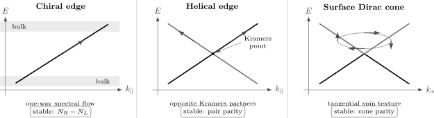
Minimal boundary spectra. Left: one chiral branch traverses the projected bulk gap and has no same-edge counterpropagating partner. Center: a helical edge contains a Kramers pair; time reversal forbids the single-particle mass that would anticross the pair. Right: a surface Dirac cone has tangential spin–pseudospin texture, so exact nonmagnetic backscattering between $\mathbf k$ and $-\mathbf k$ vanishes in the ideal single-cone model. Boundary reconstruction may add trivial pairs without changing the stable datum.

Chiral Edge Modes

A minimal charged chiral channel along coordinate $y$ has Hamiltonian

$$H_{\mathrm{ch}} = \int dy\, \psi^\dagger(y) \left( -i\hbar v\,\partial_y -\mu \right) \psi(y),$$

with dispersion

$$E(k) = \hbar vk-\mu.$$

Its group velocity has one sign:

$$v_g = \frac{1}{\hbar} \frac{\partial E}{\partial k} = v.$$

A local scalar potential can shift the phase and distort the velocity, but it cannot create elastic backscattering within an isolated one-branch theory because there is no on-shell state moving in the opposite direction on that edge.

Channel conductance

One ideal charged channel between reservoirs has conductance magnitude

$$\left| G \right| = \frac{q^2}{h}.$$

The result is independent of $v$: a slower channel carries less current per occupied state but has a proportionally larger one-dimensional density of states. Conductance Quantization owns the Landauer derivation, contacts, degeneracy factors, and imperfect transmission.

Scalar disorder as a phase shift

The absence of a counterpropagating state can be seen directly. Add a static scalar potential to one chiral branch:

$$h = -i\hbar v\,\partial_y + V(y).$$

Define

$$\psi(y) = e^{-i\vartheta(y)} \chi(y), \qquad \partial_y\vartheta = \frac{V(y)}{\hbar v}.$$

Then $h\psi=e^{-i\vartheta}(-i\hbar v\,\partial_y)\chi$. On an open edge, $V(y)$ changes only the accumulated phase. On a closed edge, it can change the boundary-condition twist and level positions, but it still supplies no reflected wave. This argument fails once another counterpropagating channel is coupled in.

For a noninteracting charge-conserving interface, an orientation can be chosen so that

$$N_R-N_L = \Delta C,$$

where $\Delta C$ is the Chern-number difference across the interface. Additional pairs can appear, but they change $N_R$ and $N_L$ equally and leave the net chirality fixed.

Why chirality is not perfect isolation

Real edges can contain:

• several co-propagating channels;
• reconstructed counterpropagating pairs;
• neutral modes;
• compressible strips from electrostatics;
• contacts that fail to equilibrate all channels;
• tunneling to the opposite edge in a narrow sample;
• bulk puddles or metallic parallel paths.

Chirality forbids Anderson localization of one isolated channel by static elastic disorder. It does not prevent energy relaxation, dephasing, interchannel equilibration, leakage into contacts, or backscattering through a remote counterpropagating sector.

Fractional and Majorana edges

An interacting Laughlin edge is not a free electron band. Its low-energy field is a chiral boson, and electron and quasiparticle operators have interaction-specific scaling dimensions. Edge reconstruction and long-range Coulomb coupling can change nonuniversal exponents without changing the bulk topological order. Fractional Quantum Hall Effect owns the action, charge normalization, tunneling laws, and equilibration caveats.

A chiral Majorana channel instead obeys $\gamma^\dagger=\gamma$ and has

$$H_{\mathrm{M}} = \frac{i\hbar v}{2} \int dy\, \gamma(y)\partial_y\gamma(y).$$

It carries heat but no conserved electrical charge and contributes chiral central charge $1/2$. Electrical conductance is therefore the wrong universal probe. These two examples show why “edge mode” does not imply “ordinary one-electron channel.”

Helical Edge Modes

A helical edge contains counterpropagating partners related by time reversal. In the basis

$$\Psi = \begin{pmatrix} \psi_R\\ \psi_L \end{pmatrix},$$

a minimal theory is

$$H_0 = \int dy\, \Psi^\dagger \left( -i\hbar v\,\sigma_z\partial_y -\mu \right) \Psi.$$

The branches have dispersions

$$E_\pm(k) = \pm\hbar vk-\mu.$$

Time reversal exchanges them. At a time-reversal-invariant momentum, Kramers theorem forces a degeneracy.

The forbidden mass

A single-particle gap requires a matrix that anticommutes with $\sigma_z$:

$$H_m = \int dy\, \Psi^\dagger \left( m_x\sigma_x + m_y\sigma_y \right) \Psi.$$

For a spin-half Kramers pair,

$$\Theta\sigma_i\Theta^{-1} = -\sigma_i.$$

Therefore constant $m_x$ and $m_y$ break time reversal. A scalar potential $V(y)I$ preserves it and cannot open a clean single-particle gap at the Kramers crossing.

This statement concerns one anomalous Kramers pair. Two pairs can be mixed and gapped by time-reversal-symmetric couplings. The stable datum is the parity of the pair count, not the visibility of every crossing in a particular surface band plot.

Kramers backscattering

Let $\lvert u\rangle$ be one state and $\Theta\lvert u\rangle$ its counterpropagating partner. For a Hermitian perturbation $V$ satisfying

$$\Theta V\Theta^{-1} = V,$$

the direct matrix element is

$$M = \langle \Theta u \rvert V \lvert u \rangle.$$

Using antiunitarity, $[V,\Theta]=0$, and $\Theta^2=-1$,

$$\begin{aligned} M &= \langle \Theta(Vu) \rvert \Theta(\Theta u) \rangle\\ &= - \langle V\Theta u \rvert u \rangle\\ &= -M. \end{aligned}$$

Hence $M=0$. This is the precise nonmagnetic single-particle backscattering statement at a Kramers pair.

Helical does not mean conserved spin

In an idealized spin-conserving model one may label the branches $\uparrow$ and $\downarrow$. Generic spin–orbit coupling rotates the spin texture with momentum and orbital composition. The robust statement is Kramers locking:

$$\lvert u_{-\mathbf k}\rangle \propto \Theta \lvert u_{\mathbf k}\rangle,$$

not a momentum-independent eigenvalue of $S_z$.

This distinction matters experimentally. Spin-resolved spectroscopy can find reduced polarization because the measured electron spin is entangled with orbitals, the photoemission matrix element is selective, and the boundary state can hybridize with trivial bands. None of those observations alone destroys the $\mathbb Z_2$ boundary anomaly.

Interactions and inelastic processes

Time reversal forbids one elastic backscattering event between one Kramers pair. It does not forbid every many-body process. Allowed mechanisms can include:

• two-particle backscattering;
• inelastic backscattering through interactions and disorder;
• Kondo scattering from a magnetic impurity;
• coupling to nuclear spins or fluctuating moments;
• spontaneous time-reversal breaking at strong coupling;
• tunneling between opposite edges.

A helical Luttinger liquid is described by

$$H_{\mathrm{HLL}} = \frac{\hbar u}{2\pi} \int dy\, \left[ K \left( \partial_y\theta \right)^2 + \frac{1}{K} \left( \partial_y\phi \right)^2 \right].$$

The Luttinger parameter $K$ controls the scaling of multiparticle operators. Whether an allowed process becomes relevant depends on interaction strength, commensuration, disorder structure, and whether the perturbation is local or extended. “Time reversal is present” is therefore not a complete transport model.

Ideal conductance and finite length

One ideal helical edge gives conductance magnitude $e^2/h$ between reservoirs. A short two-terminal bar with two equivalent edges can approach $2e^2/h$. Deviations can come from contact resistance, bulk leakage, edge puddles, inelastic scattering, nonuniform gating, or insufficiently short length.

A useful experimental hierarchy is:

1. show conduction persists when the two-dimensional bulk is depleted;
2. demonstrate edge rather than area scaling;
3. test nonlocal response consistent with the perimeter network;
4. vary edge length and temperature;
5. test sensitivity to time-reversal breaking;
6. compare several device geometries and contacts.

A conductance value near $2e^2/h$ on one device is compatible with helical edges, not a self-contained proof.

Surface Dirac Cones

For a surface normal to $\hat{\mathbf z}$, the minimal strong-topological-insulator Hamiltonian is

$$H_D(\mathbf k) = \hbar v_D \left( k_x\sigma_y - k_y\sigma_x \right) - \mu.$$

Its energies are

$$E_\pm(\mathbf k) = \pm \hbar v_D \lvert\mathbf k\rvert - \mu.$$

For the ideal isotropic model, the pseudospin expectation is tangential to the constant-energy contour:

$$\langle \boldsymbol\sigma \rangle_\pm = \pm \frac{ \hat{\mathbf z} \times \mathbf k }{ \lvert\mathbf k\rvert }.$$

This is spin–momentum locking in the effective model. Crystal orbitals and spin–orbit entanglement can reduce or tilt the measured physical-spin polarization.

Time-reversal-breaking mass

The mass term

$$H_{\mathrm{gap}} = m\sigma_z$$

produces

$$E_\pm(\mathbf k) = \pm \sqrt{ \hbar^2v_D^2 \lvert\mathbf k\rvert^2 + m^2 } - \mu.$$

Because $\Theta\sigma_z\Theta^{-1}=-\sigma_z$, this mass breaks time reversal and opens a gap $2\lvert m\rvert$ at the Dirac point. A perpendicular exchange field is one possible source. Structural asymmetry, scalar disorder, and ordinary surface potentials can shift or warp the cone but cannot generate this mass in a single isolated time-reversal-symmetric Dirac theory.

The converse needs care: a spectroscopic gap at the nominal Dirac energy does not by itself prove magnetic mass generation. Hybridization between opposite surfaces, finite momentum resolution, matrix-element suppression, band bending, disorder, or overlap with bulk bands can mimic or obscure a gap.

Warping without gapping

Crystal symmetry permits corrections. On a threefold surface, a common term is

$$H_w = \frac{\lambda}{2} \left( k_+^3+k_-^3 \right) \sigma_z, \qquad k_\pm=k_x\pm ik_y.$$

The cubic momentum factor and $\sigma_z$ are both odd under time reversal, so their product is invariant. It distorts circular constant-energy contours into hexagonal or snowflake-like shapes and introduces an out-of-plane spin component, but it does not create a mass at $\mathbf k=0$.

Exact backscattering versus general scattering

For an ideal single cone, states at $\mathbf k$ and $-\mathbf k$ are Kramers partners. The matrix element of a time-reversal-invariant scalar impurity between them vanishes:

$$\langle u_{-\mathbf k} \rvert V \lvert u_{\mathbf k} \rangle = 0.$$

This removes the exact $180^\circ$ elastic event in first order. It does not remove:

• scattering through other angles;
• small-angle momentum relaxation;
• multistep processes;
• scattering between multiple pockets or trivial surface bands;
• magnetic or spin-dependent disorder;
• electron–electron and electron–phonon processes;
• leakage into bulk states.

Weak antilocalization and characteristic quasiparticle-interference patterns can follow, but “no backscattering” should never be translated into “infinite conductivity.”

Thin films and paired surfaces

A thick three-dimensional sample has spatially separated top and bottom surfaces. In a thin film, their wavefunctions overlap. A minimal two-surface model adds a pseudospin $\boldsymbol\tau$ and a hybridization mass such as

$$H_{\mathrm{film}} = \hbar v_D \left( k_x\sigma_y-k_y\sigma_x \right) \tau_z + m_h\tau_x.$$

The term $m_h\tau_x$ preserves time reversal but gaps the pair of cones. Its magnitude typically decays as

$$\lvert m_h(d)\rvert \sim m_0 \exp\!\left( -\frac{d}{\xi} \right),$$

possibly with model-dependent oscillations. This does not contradict protection of one isolated surface: the finite film supplies a second anomalous surface that cancels the first.

Odd and even cone counts

An odd number of Dirac cones is stable under time reversal and charge conservation at the surface of a strong topological insulator. Ordinary surface bands can add cones in pairs. Consequently:

• counting every visible crossing is less reliable than tracking connectivity across the bulk gap;
• two nearby cones can mix and gap without breaking time reversal;
• a cone can merge into the projected bulk continuum and re-emerge elsewhere;
• surface reconstruction can fold the Brillouin zone;
• a weak topological insulator can have orientation-dependent “dark” surfaces.

For interacting three-dimensional SPT phases, a symmetric surface may also gap by developing intrinsic topological order. Symmetry-Protected Topological Phases owns that anomaly and boundary-option ledger.

Other Boundary Families

The chiral, helical, and Dirac models are organizing templates, not the whole subject.

Majorana boundaries

BdG particle–hole redundancy permits self-conjugate boundary quasiparticles. Depending on dimension and symmetry class, a topological superconductor can support end Majoranas, a helical or chiral Majorana edge, or a Majorana surface cone. These states are charge neutral in the quasiparticle sense, so tunneling, Andreev reflection, thermal transport, parity, and nonlocal consistency replace ordinary channel conductance as the central probes.

Fermi arcs

A Weyl-semimetal surface can host an open constant-energy contour. The arc is assembled from chiral edge states of two-dimensional momentum slices whose Chern number is nonzero. Its shape is termination dependent; its endpoints merge into projected bulk Weyl nodes. If opposite charges project to the same surface momentum, the arc can disappear on that face.

Interacting topological boundaries

Intrinsic topological order can support boundaries selected by anyon condensation. Different boundaries of the same bulk can be gapless, gapped, or separated by localized defect modes. The bulk fixes which condensates and anomalies are allowed, not one microscopic dispersion. Topological Order owns this classification and its chiral-central-charge constraints.

Robustness and Symmetry

Protection is always conditional. A useful question is not “Is the boundary robust?” but:

Which local perturbations are allowed, which stable boundary datum do they preserve, and what alternative low-energy boundary can they produce?

Perturbation ledger

Perturbation	Chiral edge	Helical edge	Strong-TI surface
smooth scalar potential	shifts phase and velocity	preserves Kramers crossing	shifts or warps spectrum
nonmagnetic static disorder	no localization for one isolated chiral channel	forbids direct one-particle Kramers backscattering	forbids exact $\mathbf k\to-\mathbf k$ event for one cone
magnetic order or field	changes details; net chirality remains while bulk phase remains	permits a single-particle mass	permits a Dirac mass
added trivial boundary bands	adds counterpropagating pairs	adds Kramers pairs	adds even cone count or ordinary pockets
opposite-boundary overlap	enables tunneling and backscattering	opens a finite-width hybridization gap	opens a thin-film hybridization gap
interactions	reconstructs and equilibrates modes	permits multiparticle processes or symmetry breaking	renormalizes cone or enables symmetric topological order
bulk-gap closing	can change net chirality	can change pair parity	can change odd-cone anomaly

Stable data versus visible spectra

Boundary spectroscopy depends on termination. The following can change without a bulk topological transition:

$$v, \qquad \mu, \qquad \xi, \qquad \text{crossing position}, \qquad \text{extra trivial pairs}.$$

Stable information instead includes quantities such as

$$N_R-N_L, \qquad N_{\mathrm{Kramers}}\pmod2, \qquad N_{\mathrm{Dirac}}\pmod2,$$

under their appropriate assumptions.

This is why one should compare whole dispersions and symmetry representations rather than one surface band at one momentum.

Boundary reconstruction

Electrostatics and interactions can produce extra channels before the bulk gap changes. A smooth quantum Hall edge can separate into compressible and incompressible strips. A topological-insulator surface can acquire Rashba-split accumulation subbands. A fractional edge can develop counterpropagating neutral structure.

Reconstruction complicates transport and tunneling but does not automatically change the bulk. The correct workflow is:

1. identify all boundary branches, including trivial ones;
2. determine which can pair and gap under the allowed symmetry;
3. isolate the residual anomalous content;
4. model equilibration and contacts before predicting conductance.

Disorder and localization

The absence of one matrix element is weaker than immunity to disorder. Disorder can:

• broaden energy and momentum;
• create charge puddles;
• move the chemical potential through bulk bands;
• couple distant boundary segments;
• generate random magnetic regions;
• make finite-size gaps spatially nonuniform;
• alter dephasing and equilibration lengths.

Chiral channels have the strongest one-dimensional localization obstruction because no counterpropagating state exists in the isolated theory. Helical and Dirac boundaries belong to time-reversal-symmetric spin–orbit settings, where destructive interference can produce weak antilocalization, but interactions, multiple channels, symmetry breaking, and bulk leakage determine real transport.

Symmetry breaking can be local

The bulk may preserve time reversal while the surface breaks it. Magnetic coating, an applied field, a reconstructed moment, or spontaneous boundary order can gap a helical or Dirac boundary without changing the bulk phase. The resulting gapped boundary can carry its own response or domain-wall modes.

Conversely, a nominally nonmagnetic sample can experience stray fields, magnetic dopants, or proximity exchange. Experimental protection claims therefore require a boundary-specific symmetry audit, not just the bulk space group.

Experimental Probes

No single probe returns “topological boundary state” as a direct observable. Each measures a projection of the boundary spectral function, wavefunction, response, or scattering matrix.

Angle-resolved photoemission

In a sudden-approximation description,

$$I(\mathbf k,\omega) \propto \left| M_{fi} \right|^2 f(\omega) A(\mathbf k,\omega),$$

where $M_{fi}$ is a photon-energy- and polarization-dependent matrix element, $f$ is the Fermi function, and $A$ is the occupied spectral function. Photoelectron Spectroscopy owns the full measurement formalism.

For a candidate surface state, ARPES can test:

• a branch inside the projected bulk gap;
• connectivity between bulk valence and conduction sectors;
• a Dirac crossing or Fermi arc;
• weak dependence on photon-energy-inferred $k_\perp$;
• surface aging and termination dependence;
• agreement with a slab calculation.

Failure modes include matrix-element extinction, finite $k_\perp$ resolution, surface charging, adsorbates, band bending, unresolved gaps, and overlap with bulk spectral weight. A linear dispersion alone is not a topological diagnosis.

Spin-resolved photoemission

Spin-resolved ARPES tests the reversal of spin polarization around a surface contour. It supports spin–momentum locking when the momentum, band identity, and detector response are controlled.

The measured polarization need not be unity. Orbital entanglement, unresolved bands, final-state effects, domain averaging, and detector calibration matter. Conversely, a Rashba-split ordinary surface state can also have a helical-looking spin texture. The stable distinction requires bulk connectivity and crossing parity.

Scanning tunneling spectroscopy and interference

For a featureless tip at low temperature,

$$\frac{dI}{dV}(\mathbf r,V) \propto \rho_s \left( \mathbf r, E_F+qV \right).$$

Defects generate standing-wave modulations. Their Fourier transform $\delta\rho(\mathbf q,\omega)$ samples scattering between equal-energy states separated by $\mathbf q$, weighted by spinor overlap and the impurity $T$ matrix.

In an ideal helical contour, the exact vector connecting $\mathbf k$ to $-\mathbf k$ is suppressed for a scalar impurity. But a missing Fourier feature is not automatically proof of topology: matrix elements, weak impurity strength, finite field of view, orbital selection, and overlapping bands can also suppress intensity. A strong analysis predicts the complete allowed and forbidden $\mathbf q$ pattern.

Scanning Tunneling Microscopy and Spectroscopy owns the tunneling junction, setpoint normalization, Fourier-map workflow, impurity $T$ matrix, and non-topological QPI artifacts.

Electrical transport

Boundary transport is persuasive when geometry and tuning separate it from the bulk. Useful tests include:

• gating through a bulk-depleted regime;
• length, width, thickness, and perimeter scaling;
• local and nonlocal voltage configurations;
• contact permutations;
• temperature and bias dependence;
• response to controlled time-reversal breaking;
• comparison with capacitance or thermodynamic carrier density.

An approximate parallel-channel ledger is

$$G_{\mathrm{meas}} \simeq G_{\mathrm{boundary}} + G_{\mathrm{bulk}} + G_{\mathrm{other}},$$

with contacts treated separately. In three-dimensional topological insulators, residual bulk carriers often dominate even when ARPES clearly resolves a surface cone. Surface spectroscopy and surface-dominated transport are different achievements.

Thermal and neutral-mode probes

Electrical transport misses charge-neutral Majorana or fractional neutral modes. Thermal conductance, noise, upstream heat propagation, and energy equilibration can probe net chiral central charge. Interpretation requires phonon subtraction, contact calibration, and an equilibration model.

Controlled perturbations

A protection claim becomes stronger when the boundary responds selectively:

• a time-reversal-breaking perturbation gaps a helical or Dirac boundary;
• a nonmagnetic perturbation shifts or broadens it without producing the forbidden mass;
• opposite-surface hybridization decays with thickness;
• changing surface orientation modifies weak-TI or Weyl boundary visibility as predicted;
• domain walls in a boundary mass bind the expected lower-dimensional channel.

The perturbation must be characterized independently. Depositing nominally magnetic atoms can also dope, disorder, or reconstruct a surface, so a spectral change is not automatically an exchange gap.

Evidence ladder

Evidence level	What is established	What remains open
boundary-localized spectral weight	a surface or edge state exists	whether it is topological
dispersion inside a projected gap	a candidate boundary branch	trivial Tamm, Shockley, or band-bending alternatives
bulk connectivity and odd crossing parity	consistency with a bulk invariant	matrix-element and termination ambiguities
Kramers or chiral scattering selection	symmetry texture consistent with protection	full transport and bulk phase
geometry-dependent boundary transport	conduction follows edge or surface network	contacts, puddles, parallel channels
controlled symmetry-breaking response	the predicted protection condition is active	interaction and finite-size alternatives
convergent multi-probe package	robust phase-level identification	quantitative boundary reconstruction

Established and active claims

Established: chiral edge transport in integer quantum Hall systems; helical-edge evidence in several two-dimensional topological-insulator platforms; surface Dirac states in canonical three-dimensional topological insulators; spin-textured and quasiparticle-interference signatures consistent with time-reversal protection.

Material and device dependent: the length over which a helical edge remains ballistic; isolation of surface-only electrical transport; quantitative surface gaps under magnetic perturbations; fractional-edge equilibration; interaction-driven reconstruction; correspondence between one cleaved surface and device interfaces.

Not implied by boundary spectroscopy alone: dissipationless electronics, quantized spin current, room-temperature topological transport, non-Abelian statistics, or fault-tolerant computation.

Common Mistakes

Calling every in-gap surface band topological

Tamm, Shockley, dangling-bond, accumulation, and reconstruction states can lie in a projected gap. Establish connectivity, stable parity or chirality, symmetry response, and the bulk phase.

Treating protection as absence of scattering

Helical and Dirac boundaries forbid a specific Kramers backscattering matrix element. Other angles, inelastic processes, extra bands, and bulk leakage remain.

Assuming physical spin is conserved

Spin–orbit coupling makes the boundary label a Kramers pseudospin. Measured spin polarization can vary around the contour and need not be quantized.

Inferring a magnetic mass from one apparent gap

Finite thickness, avoided crossings with trivial bands, disorder, resolution, and matrix-element suppression can mimic a gap. Track thickness, magnetization, temperature, momentum dependence, and both branches.

Ignoring the projected bulk spectrum

A surface branch can merge into bulk states. Localization and visibility must be evaluated at fixed $\mathbf k_\parallel$, not from a global bulk gap alone.

Counting crossings without stable equivalence

Ordinary boundary pairs can be added or removed. Net chirality and parity are more robust than the raw number of lines in one calculation.

Using one conductance plateau as proof

Contacts, ballistic trivial channels, bulk shunts, and device inhomogeneity can produce suggestive values. Require geometry, length, gate, temperature, nonlocal, and symmetry tests.

Modeling a fractional edge as a free electron channel

Fractional edges are interacting boundary theories with charge and neutral sectors. Their scaling exponents and equilibration cannot be inferred from one-electron band velocity alone.

Forgetting opposite boundaries

Finite strips and films contain at least two sides. Their exponentially small overlap can open a gap or restore backscattering without any bulk transition.

Exercises

1. Gauge away scalar disorder in a chiral channel

For

$$h = -i\hbar v\,\partial_y + V(y),$$

show that a static scalar $V(y)$ can be removed locally by a phase redefinition. What remains on a ring of circumference $L$?

Solution

Set

$$\psi(y) = e^{-i\vartheta(y)} \chi(y), \qquad \vartheta(y) = \frac{1}{\hbar v} \int_0^y V(y')\,dy'.$$

Then

$$\begin{aligned} h\psi &= \left( -i\hbar v\,\partial_y+V \right) e^{-i\vartheta}\chi\\ &= e^{-i\vartheta} \left( -\hbar v\,\partial_y\vartheta +V -i\hbar v\,\partial_y \right) \chi\\ &= e^{-i\vartheta} \left( -i\hbar v\,\partial_y \right) \chi. \end{aligned}$$

There is no reflected branch. On a ring, periodicity of $\psi$ gives a twisted condition for $\chi$:

$$\chi(L) = \exp\!\left( i \frac{1}{\hbar v} \oint V(y)\,dy \right) \chi(0).$$

The scalar potential shifts the quantized momenta through this total phase. It does not localize the single chiral channel.

2. Classify helical-edge perturbations

For

$$h_0(k) = \hbar vk\sigma_z,$$

classify the constant perturbations $a_0I+a_x\sigma_x+a_y\sigma_y+a_z\sigma_z$ by whether they preserve time reversal and whether they open a gap.

Solution

Time reversal sends $k\to-k$ and $\sigma_i\to-\sigma_i$. The kinetic product $k\sigma_z$ is invariant.

The scalar $a_0I$ is time-reversal even. It shifts both branches and does not gap the crossing.

Each constant Pauli term is time-reversal odd. The terms $a_x\sigma_x$ and $a_y\sigma_y$ anticommute with $\sigma_z$, so either opens a gap. The term $a_z\sigma_z$ commutes with the kinetic term and shifts the two branches in momentum:

$$E_\pm(k) = \pm \left( \hbar vk+a_z \right).$$

It breaks time reversal but does not by itself create an avoided crossing in the unbounded linear model.

3. Prove Kramers backscattering vanishes

Let $\Theta^2=-1$, let $V=V^\dagger$, and suppose $[V,\Theta]=0$. Show that

$$\langle \Theta u \rvert V \lvert u \rangle = 0.$$

Solution

For antiunitary $\Theta$,

$$\langle a\rvert b\rangle = \langle \Theta b \rvert \Theta a \rangle.$$

Set $\lvert a\rangle=\Theta\lvert u\rangle$ and $\lvert b\rangle=V\lvert u\rangle$. Then

$$\begin{aligned} M &= \langle \Theta u \rvert Vu \rangle\\ &= \langle \Theta(Vu) \rvert \Theta(\Theta u) \rangle\\ &= - \langle V\Theta u \rvert u \rangle. \end{aligned}$$

Hermiticity gives

$$\langle V\Theta u \rvert u \rangle = \langle \Theta u \rvert V \lvert u \rangle = M.$$

Thus $M=-M$, so $M=0$. The proof fails if $\Theta^2=+1$ or if $V$ breaks time reversal.

4. Spin texture of a surface Dirac cone

For

$$H_D = \hbar v_D \left( k_x\sigma_y-k_y\sigma_x \right),$$

find the energies and pseudospin direction of the upper cone. What is the pseudospin overlap between $\mathbf k$ and $-\mathbf k$?

Solution

Write

$$H_D = \mathbf d(\mathbf k) \cdot \boldsymbol\sigma, \qquad \mathbf d = \hbar v_D \left( -k_y,k_x,0 \right).$$

The energies are

$$E_\pm = \pm \lvert\mathbf d\rvert = \pm \hbar v_D \lvert\mathbf k\rvert.$$

The upper-cone eigenstate has

$$\langle \boldsymbol\sigma \rangle_+ = \frac{\mathbf d}{\lvert\mathbf d\rvert} = \frac{ \hat{\mathbf z}\times\mathbf k }{ \lvert\mathbf k\rvert }.$$

At $-\mathbf k$ the pseudospin reverses. The two normalized spinors are orthogonal:

$$\left| \langle u_+(-\mathbf k) \rvert u_+(\mathbf k) \rangle \right|^2 = 0.$$

That orthogonality suppresses exact scalar backscattering in the minimal model.

5. Magnetic gap or thin-film hybridization?

Two samples show a $12\,\mathrm{meV}$ gap near a surface Dirac point. In sample A the gap decreases exponentially as film thickness grows and remains at zero applied magnetization. In sample B it is thickness independent above $20\,\mathrm{nm}$ and follows the perpendicular magnetization. Identify the leading interpretation of each and name one additional check.

Solution

Sample A is consistent with top–bottom surface hybridization. The paired surfaces can gap while preserving time reversal, and their overlap decays exponentially with thickness. A useful check is to compare the decay length with the calculated surface penetration depth or to look for opposite-surface wavefunction weight.

Sample B is consistent with a time-reversal-breaking exchange mass. A useful check is to reverse magnetization and test the associated Hall or domain-wall response, while separately measuring chemical-potential shifts and surface reconstruction.

Neither assignment follows from the gap alone. ARPES resolution, disorder, avoided crossings with trivial bands, and band bending must be excluded.

6. Extract a boundary penetration depth

A symmetric topological-insulator film has hybridization gaps

$$\Delta(d) = \Delta_0e^{-d/\xi}.$$

Measurements give $\Delta(6\,\mathrm{nm})=20\,\mathrm{meV}$ and $\Delta(10\,\mathrm{nm})=5\,\mathrm{meV}$. Estimate $\xi$.

Solution

Taking the ratio eliminates $\Delta_0$:

$$\frac{ \Delta(6) }{ \Delta(10) } = \exp\!\left( \frac{4\,\mathrm{nm}}{\xi} \right) = 4.$$

Therefore

$$\xi = \frac{ 4\,\mathrm{nm} }{ \ln4 } \approx 2.89\,\mathrm{nm}.$$

With more thicknesses one should fit the full data and test for oscillations or multiple decay lengths rather than trusting a two-point estimate.

7. Audit a quasiparticle-interference claim

An STM Fourier map lacks intensity at one vector close to $2k_F$. The authors call this proof of a topological surface state. What further information is required?

Solution

A missing vector can result from spinor orthogonality, but also from impurity form factors, orbital matrix elements, weak scattering, limited field of view, energy resolution, or overlap with another band.

A stronger analysis should provide:

• the measured or calculated constant-energy contour;
• the full joint-density and spin-selective scattering calculation;
• impurity character and a $T$-matrix model;
• energy evolution of all predicted $\mathbf q$ vectors;
• comparison with spin-resolved ARPES;
• evidence that the band connects the projected bulk valence and conduction sectors;
• response to magnetic versus nonmagnetic scatterers.

The missing feature is compatible with Kramers protection but is not a phase diagnosis by itself.

8. Evaluate a boundary-transport claim

A three-dimensional crystal has an ARPES Dirac cone and a low-temperature sheet resistance that saturates. Hall data show a carrier density that changes little with gate voltage, and the sample thickness has not been varied. The saturation is called “dissipationless topological surface transport.” Evaluate the claim and design a stronger test set.

Solution

ARPES establishes a candidate topological surface band on the cleaved surface. Resistance saturation only establishes a residual conduction channel. Bulk defects, impurity bands, side surfaces, an accumulation layer, contact shunts, and electron–hole puddles remain possible. Finite resistance is also not dissipationless transport.

A stronger program would:

1. gate through the surface Dirac point while independently tracking capacitance or carrier density;
2. vary thickness to separate volume and surface conductance;
3. compare local and nonlocal geometries;
4. fit multichannel Hall and longitudinal data over field and temperature;
5. use quantum oscillations with angular dependence;
6. verify surface localization on the actual device interface;
7. test weak-field interference and controlled magnetic perturbations;
8. reproduce the result across contacts and samples.

The justified conclusion is “surface states are spectroscopically established and may contribute to residual transport,” not dissipationless surface-only conduction.

Connections

• Topology in Quantum Matter supplies the phase-equivalence, invariant, response, and evidence framework.
• Bulk–Boundary Correspondence owns relative bulk indices, oriented mode counting, domain-wall solutions, anomaly matching, and strip numerics.
• Angle-Resolved Photoemission Spectroscopy develops photon-energy, polarization, surface-termination, matrix-element, and line-shape controls for boundary-band claims.
• Integer Quantum Hall Effect develops chiral charged edges in Hall bars, including localization, contacts, and metrology.
• Fractional Quantum Hall Effect owns fractional edge theories, neutral modes, tunneling, equilibration, and thermal evidence.
• Topological Insulators owns quantum spin Hall bulk indices, three-dimensional strong and weak indices, and material-specific evidence.
• Topological Superconductors owns Majorana end, edge, surface, and vortex states together with experimental claim audits.
• Weyl and Dirac Semimetals owns surface Fermi arcs and their projected-node constraints.
• Symmetry-Protected Topological Phases explains boundary anomalies, interacting gapping options, and symmetry-preserving topological order.
• Topological Order develops anyon condensation, chiral central charge, and allowed boundaries of intrinsic order.
• Time Reversal for Spin One-Half and Kramers Degeneracy supply the antiunitary algebra behind helical protection.
• Conductance Quantization and Mesoscopic Transport own the reservoir, contact, scattering-matrix, and nonlocal-transport machinery.
• Spectral Functions supplies the many-body meaning of boundary spectral weight and linewidth.
• Photoelectron Spectroscopy develops the photoemission observable, matrix elements, and resolution.

Further Reading

• M. Z. Hasan and C. L. Kane, “Colloquium: Topological Insulators,” Reviews of Modern Physics 82, 3045–3067 (2010), doi:10.1103/RevModPhys.82.3045.
• X.-L. Qi and S.-C. Zhang, “Topological Insulators and Superconductors,” Reviews of Modern Physics 83, 1057–1110 (2011), doi:10.1103/RevModPhys.83.1057.
• B. A. Bernevig and T. L. Hughes, Topological Insulators and Topological Superconductors, Princeton University Press, 2013.
• M. Stone, ed., Quantum Hall Effect, World Scientific, 1992.

References

Boundary states and chiral edges

1. W. Shockley, “On the Surface States Associated with a Periodic Potential,” Physical Review 56, 317–323 (1939), doi:10.1103/PhysRev.56.317.
2. B. I. Halperin, “Quantized Hall Conductance, Current-Carrying Edge States, and the Existence of Extended States in a Two-Dimensional Disordered Potential,” Physical Review B 25, 2185–2190 (1982), doi:10.1103/PhysRevB.25.2185.
3. M. Büttiker, “Absence of Backscattering in the Quantum Hall Effect in Multiprobe Conductors,” Physical Review B 38, 9375–9389 (1988), doi:10.1103/PhysRevB.38.9375.
4. X.-G. Wen, “Chiral Luttinger Liquid and the Edge Excitations in the Fractional Quantum Hall States,” Physical Review B 41, 12838–12844 (1990), doi:10.1103/PhysRevB.41.12838.
5. Y. Hatsugai, “Chern Number and Edge States in the Integer Quantum Hall Effect,” Physical Review Letters 71, 3697–3700 (1993), doi:10.1103/PhysRevLett.71.3697.

Helical edges and time-reversal protection

6. C. L. Kane and E. J. Mele, “Quantum Spin Hall Effect in Graphene,” Physical Review Letters 95, 226801 (2005), doi:10.1103/PhysRevLett.95.226801.
7. C. L. Kane and E. J. Mele, “$\mathbb Z_2$ Topological Order and the Quantum Spin Hall Effect,” Physical Review Letters 95, 146802 (2005), doi:10.1103/PhysRevLett.95.146802.
8. C. Wu, B. A. Bernevig, and S.-C. Zhang, “Helical Liquid and the Edge of Quantum Spin Hall Systems,” Physical Review Letters 96, 106401 (2006), doi:10.1103/PhysRevLett.96.106401.
9. C. Xu and J. E. Moore, “Stability of the Quantum Spin Hall Effect: Effects of Interactions, Disorder, and $\mathbb Z_2$ Topology,” Physical Review B 73, 045322 (2006), doi:10.1103/PhysRevB.73.045322.
10. B. A. Bernevig, T. L. Hughes, and S.-C. Zhang, “Quantum Spin Hall Effect and Topological Phase Transition in HgTe Quantum Wells,” Science 314, 1757–1761 (2006), doi:10.1126/science.1133734.
11. M. König et al., “Quantum Spin Hall Insulator State in HgTe Quantum Wells,” Science 318, 766–770 (2007), doi:10.1126/science.1148047.
12. Z. Fei et al., “Edge Conduction in Monolayer $\mathrm{WTe_2}$,” Nature Physics 13, 677–682 (2017), doi:10.1038/nphys4091.
13. S. Wu et al., “Observation of the Quantum Spin Hall Effect up to 100 Kelvin in a Monolayer Crystal,” Science 359, 76–79 (2018), doi:10.1126/science.aan6003.

Surface Dirac cones and probes

14. L. Fu, C. L. Kane, and E. J. Mele, “Topological Insulators in Three Dimensions,” Physical Review Letters 98, 106803 (2007), doi:10.1103/PhysRevLett.98.106803.
15. J. E. Moore and L. Balents, “Topological Invariants of Time-Reversal-Invariant Band Structures,” Physical Review B 75, 121306(R) (2007), doi:10.1103/PhysRevB.75.121306.
16. X.-L. Qi, T. L. Hughes, and S.-C. Zhang, “Topological Field Theory of Time-Reversal Invariant Insulators,” Physical Review B 78, 195424 (2008), doi:10.1103/PhysRevB.78.195424.
17. D. Hsieh et al., “A Topological Dirac Insulator in a Quantum Spin Hall Phase,” Nature 452, 970–974 (2008), doi:10.1038/nature06843.
18. H. Zhang et al., “Topological Insulators in $\mathrm{Bi_2Se_3}$, $\mathrm{Bi_2Te_3}$ and $\mathrm{Sb_2Te_3}$ with a Single Dirac Cone on the Surface,” Nature Physics 5, 438–442 (2009), doi:10.1038/nphys1270.
19. Y. Xia et al., “Observation of a Large-Gap Topological-Insulator Class with a Single Dirac Cone on the Surface,” Nature Physics 5, 398–402 (2009), doi:10.1038/nphys1274.
20. D. Hsieh et al., “A Tunable Topological Insulator in the Spin Helical Dirac Transport Regime,” Nature 460, 1101–1105 (2009), doi:10.1038/nature08234.
21. Y. L. Chen et al., “Experimental Realization of a Three-Dimensional Topological Insulator, $\mathrm{Bi_2Te_3}$,” Science 325, 178–181 (2009), doi:10.1126/science.1173034.
22. L. Fu, “Hexagonal Warping Effects in the Surface States of the Topological Insulator $\mathrm{Bi_2Te_3}$,” Physical Review Letters 103, 266801 (2009), doi:10.1103/PhysRevLett.103.266801.
23. P. Roushan et al., “Topological Surface States Protected from Backscattering by Chiral Spin Texture,” Nature 460, 1106–1109 (2009), doi:10.1038/nature08308.
24. Z. Alpichshev et al., “STM Imaging of Electronic Waves on the Surface of $\mathrm{Bi_2Te_3}$: Topologically Protected Surface States and Hexagonal Warping Effects,” Physical Review Letters 104, 016401 (2010), doi:10.1103/PhysRevLett.104.016401.
25. D. Kim et al., “Surface Conduction of Topological Dirac Electrons in Bulk Insulating $\mathrm{Bi_2Se_3}$,” Nature Physics 8, 459–463 (2012), doi:10.1038/nphys2286.