Conductance Quantization

Conductance quantization is the appearance of reproducible conductance plateaus when a narrow ballistic conductor opens one propagating transverse mode at a time. A perfectly transmitted, nondegenerate channel contributes

$$g_q = \frac{e^2}{h},$$

where $e>0$ is the elementary charge. If each orbital mode has two unresolved spin states, the step is instead the conventional conductance quantum

$$G_0 \equiv \frac{2e^2}{h}.$$

The integer is therefore a count of transmitting channels, including whatever spin, valley, layer, edge, or other internal labels remain distinct. It is not a quantization of bulk conductivity and it does not imply that every microscopic transmission probability is exactly one.

This page is the canonical home for the plateau phenomenon and its experimental diagnosis: channel counting, degeneracy, imperfect transmission, thermal and finite-bias rounding, contact resistance, and evidence from semiconductor and atomic constrictions. Quantum Point Contacts owns split-gate electrostatics, local adiabatic modes, pinch-off maps, charge sensing, bandwidth, and detector backaction. Reflection and Transmission Coefficients owns elementary current-based scattering conventions, Mesoscopic Transport owns master equations and counting statistics, and Integer Quantum Hall Effect owns topological edge-channel quantization.

Use the Transport, Response, and Optics gateway when deciding between a bulk coefficient and a coherent-terminal description.

Convention Ledger

Symbol	Meaning
$e>0$	magnitude of the electron charge; an electron has charge $-e$
$V=(\mu_S-\mu_D)/e$	source–drain voltage convention used below
$a$	one resolved incoming channel, including internal labels
$T_a(E)$	transmission eigenvalue of channel $a$, with $0\le T_a\le1$
$N$	number of open orbital modes when spin is counted separately
$g_{\mathrm d}$	unresolved degeneracy carried by each orbital mode
$g_q=e^2/h$	conductance per perfectly transmitted resolved channel
$G_0=2e^2/h$	conventional spin-degenerate conductance quantum

Since the 2019 SI fixes both $e$ and $h$, these conductance scales are exact consequences of the defining constants:

$$\begin{aligned} \frac{e^2}{h} &= 38.740\,458\,649\ldots\ \mu\mathrm S, \\ G_0 &= 77.480\,917\,299\ldots\ \mu\mathrm S, \\ \frac{h}{e^2} &= 25\,812.807\,459\ldots\ \Omega, \\ \frac{h}{2e^2} &= 12\,906.403\,730\ldots\ \Omega. \end{aligned}$$

The decimals are not the experimental accuracy of a particular constriction. Device quantization is limited by transmission, temperature, contacts, calibration, interactions, and noise.

What Is Quantized?

The measured linear conductance is

$$G = \left. \frac{dI}{dV} \right|_{V=0}.$$

It relates a terminal current to a terminal voltage. Conductivity $\sigma$, by contrast, is a local or bulk constitutive coefficient. In a short coherent constriction, assigning a local electric field and a geometry-independent resistivity is generally less useful than specifying reservoirs, modes, and transmission.

For ideal resolved channels at zero temperature,

$$G = \frac{e^2}{h}N_{\mathrm{res}},$$

where $N_{\mathrm{res}}$ counts every spin or other internal branch separately. If $N$ counts orbital modes and each has the same degeneracy $g_{\mathrm d}$,

$$G = g_{\mathrm d} \frac{e^2}{h}N.$$

The staircase is quantized because $N$ changes discretely. Gate voltage itself is not quantized, and plateau widths in gate voltage are not universal.

Regime and Scale Hierarchy

A clean conductance staircase needs more than a narrow wire. Let $L_c$ and $W_c$ be the length and minimum width of the constriction, $\lambda_F$ the Fermi wavelength, $\ell_{\mathrm e}$ the elastic mean free path, $\ell_{\mathrm{in}}$ the inelastic length, and $L_\phi$ the phase-coherence length. A useful hierarchy is

$$W_c \sim \lambda_F, \qquad L_c \ll \ell_{\mathrm e},\ell_{\mathrm{in}}, \qquad k_{\mathrm B}T,\ e|V| \ll \Delta_\perp,$$

where $\Delta_\perp$ is a typical transverse-subband spacing. Coherent interference across a larger circuit additionally requires $L_\phi$ to exceed the relevant path length.

These conditions separate several ideas that are often merged:

• quantum confinement discretizes transverse motion;
• ballistic transport suppresses scattering inside the constriction;
• adiabatic opening suppresses reflection and unwanted mode conversion at the entrances;
• equilibrated reservoirs supply Fermi occupations and absorb outgoing carriers;
• low temperature and bias resolve adjacent thresholds.

Ballistic does not mean perfectly transmitted. An abrupt but impurity-free constriction can reflect strongly.

Why One Channel Gives e²/h

Consider one right-moving, nondegenerate branch with dispersion $E(k)$. In a segment of length $L$, the number of states in $dk$ is

$$dN_+ = \frac{L}{2\pi}\,dk.$$

The group velocity is

$$v(k) = \frac{1}{\hbar} \frac{dE}{dk}.$$

The density of right-moving states per unit length and energy is therefore

$$\frac{1}{L} \frac{dN_+}{dE} = \frac{1}{h\,v(E)}.$$

Each occupied state transports charge magnitude $e$ at speed $v$. The velocity cancels the one-dimensional density of states:

$$e\,v(E) \frac{1}{h\,v(E)} dE = \frac{e}{h}\,dE.$$

If the source and drain inject distributions $f_S(E)$ and $f_D(E)$ through a channel of transmission $T(E)$, the conventional current from source to drain is

$$I = \frac{e}{h} \int_{-\infty}^{\infty} dE\, T(E) \left[ f_S(E)-f_D(E) \right].$$

For many resolved channels,

$$I = \frac{e}{h} \sum_a \int_{-\infty}^{\infty} dE\, T_a(E) \left[ f_S(E)-f_D(E) \right].$$

Linearizing about a common chemical potential $\mu$ gives

$$G(T) = \frac{e^2}{h} \sum_a \int_{-\infty}^{\infty} dE\, T_a(E) \left( -\frac{\partial f}{\partial E} \right).$$

At zero temperature, $-\partial f/\partial E\to\delta(E-E_F)$, so

$$G(0) = \frac{e^2}{h} \sum_a T_a(E_F).$$

The result does not depend on a parabolic dispersion. The cancellation works for any monotonic propagating branch with well-defined flux normalization. Details of the band structure determine how many branches reach $E_F$ and how well each one transmits.

Channel Counting in a Constriction

For a two-dimensional effective-mass Hamiltonian,

$$H = -\frac{\hbar^2}{2m^*} \left( \partial_x^2+\partial_y^2 \right) + U(x,y),$$

one can solve the transverse problem at fixed $x$:

$$\left[ -\frac{\hbar^2}{2m^*}\partial_y^2 + U(x,y) \right] \phi_n(y;x) = \varepsilon_n(x)\phi_n(y;x).$$

Each $\varepsilon_n(x)$ acts approximately as a longitudinal barrier. Define its bottleneck threshold by

$$E_n^* = \max_x \varepsilon_n(x).$$

The $n$th orbital channel is open when

$$E_F > E_n^*.$$

For a hard-wall guide of width $W$,

$$\varepsilon_n^\perp = \frac{\hbar^2\pi^2n^2} {2m^*W^2}, \qquad n=1,2,\ldots$$

and the zero-temperature orbital count is

$$N = \left\lfloor \frac{k_FW}{\pi} \right\rfloor.$$

The approximation becomes local when $W=W(x)$ changes slowly. A useful measure of nonadiabatic mixing is

$$\eta_{mn}(x) = \frac{ \left| \hbar v_x \langle\phi_m\vert\partial_x\phi_n\rangle \right| }{ \left| \varepsilon_m-\varepsilon_n \right| }.$$

When $\eta_{mn}\ll1$ for relevant mode pairs, a carrier follows its transverse mode through the constriction. Abrupt walls, disorder, resonances, and sharp electrostatic structure increase reflection or mode mixing.

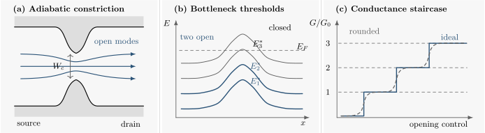
The channel-counting ledger. A smooth constriction maps each transverse mode to an effective threshold $E_n^*$ at the bottleneck. Modes below $E_F$ transmit, and each spin-degenerate orbital mode ideally raises the conductance by $G_0=2e^2/h$. Rounded risers encode finite transmission width and thermal or bias averaging; the horizontal axis is an opening control, not a universal voltage scale.

Ideal and Nonideal Steps

The sharpest idealization is

$$T_n(E) = \Theta(E-E_n^*).$$

For $g_{\mathrm d}$ degenerate internal branches,

$$G = g_{\mathrm d} \frac{e^2}{h} \sum_n \Theta(E_F-E_n^*).$$

Real transmission eigenvalues are the eigenvalues of $t^\dagger t$, where $t$ is the transmission block of the scattering matrix:

$$t^\dagger t \lvert a\rangle = T_a \lvert a\rangle, \qquad 0\le T_a\le1.$$

This basis matters when geometrical modes mix. The conductance still depends only on

$$\operatorname{Tr} \left( t^\dagger t \right) = \sum_a T_a.$$

Relative to an ideal set of $N_{\mathrm{res}}$ open channels, the deficit is

$$\Delta G = \frac{e^2}{h} \sum_{a=1}^{N_{\mathrm{res}}} \left( 1-T_a \right).$$

Quantization is therefore accurate when the open transmission eigenvalues cluster near one and the closed ones near zero. Mode mixing alone is not fatal; backscattering and partially open eigenchannels are.

Saddle-Point Model

A split-gate quantum point contact is often modeled near its bottleneck by

$$U(x,y) = U_0 -\frac12m^*\omega_x^2x^2 +\frac12m^*\omega_y^2y^2.$$

The transverse thresholds are

$$E_n = U_0 +\hbar\omega_y \left( n+\frac12 \right), \qquad n=0,1,2,\ldots$$

while the inverted longitudinal parabola gives the transmission

$$T_n(E) = \frac{1}{ 1+ \exp\!\left[ -\dfrac{2\pi(E-E_n)} {\hbar\omega_x} \right] }.$$

The intrinsic 10–90 percent energy width of one riser is

$$\Delta E_{10\text{–}90}^{\mathrm{saddle}} = \frac{\hbar\omega_x}{\pi} \ln 9.$$

Clear plateaus require the transverse spacing to exceed the combined broadening scales:

$$\hbar\omega_y \gg \max \left( k_{\mathrm B}T,\, e|V|,\, \hbar\omega_x \right)$$

as an order-of-magnitude criterion. Numerical factors depend on the chosen resolution standard.

The saddle is a local model, not a universal fit function. Self-consistent electrostatics, exchange and correlation, disorder, source–drain asymmetry, and finite thickness can all move or reshape the thresholds.

Spin and Other Degeneracies

Every resolved branch contributes $e^2/h$ when perfectly transmitted. Common plateau spacings follow from how branches are grouped:

Channel ledger	Ideal increment
one resolved branch	$e^2/h$
one orbital mode with unresolved spin degeneracy	$2e^2/h$
one mode with unresolved spin and valley degeneracy	$4e^2/h$
split spin or valley branches	separate $e^2/h$ contributions

For a simple Zeeman model,

$$E_{n,s} = E_n +s\frac{g^*\mu_{\mathrm B}B}{2}, \qquad s=\pm1.$$

As the splitting becomes larger than temperature and intrinsic width,

$$\lvert g^*\rvert\mu_{\mathrm B}B \gtrsim \max \left( k_{\mathrm B}T,\, \delta E_{\mathrm{step}} \right),$$

the usual $2e^2/h$ riser can separate into two $e^2/h$ risers. Orbital magnetic effects and field-dependent electrostatics must be separated from Zeeman splitting.

Degeneracy should never be inserted twice. If $a$ already labels spin and valley, do not multiply the channel sum by another $g_{\mathrm d}$.

Temperature and Finite Bias

Temperature does not change the zero-temperature quantum per open channel; it averages transmission over an energy window of order $k_{\mathrm B}T$. For an ideal threshold,

$$G(T) = \frac{e^2}{h} \sum_a \frac{1}{ 1+ \exp\!\left[ \dfrac{E_a^*-\mu} {k_{\mathrm B}T} \right] }.$$

The 10–90 percent thermal width is

$$\Delta E_{10\text{–}90}^{T} = 2k_{\mathrm B}T\ln9 \simeq 4.394\,k_{\mathrm B}T.$$

Gate sweeps measure this width only after an energy lever arm is established. If a threshold varies locally as

$$\delta E_n = -\alpha_g e\,\delta V_g,$$

then $\alpha_g$ can convert gate voltage to energy, but it may depend on gate setting and device geometry.

At finite source–drain bias with symmetric electrochemical potentials,

$$\mu_S = \mu+\frac{eV}{2}, \qquad \mu_D = \mu-\frac{eV}{2},$$

the differential conductance is

$$\frac{dI}{dV} = \frac{e^2}{2h} \sum_a \int dE\, T_a(E) \left[ -\frac{\partial f_S}{\partial E} -\frac{\partial f_D}{\partial E} \right].$$

At zero temperature,

$$\frac{dI}{dV} = \frac{e^2}{2h} \sum_a \left[ T_a(\mu_S) + T_a(\mu_D) \right].$$

A threshold lying between $\mu_D$ and $\mu_S$ can therefore give a half-step in the symmetric idealization. Finite-bias transconductance maps can determine subband spacings, but only after checking where the voltage drops and whether heating or nonlinear electrostatics matter.

Contact Resistance and Dissipation

A perfectly transmitted channel has no elastic backscattering in the constriction, yet a two-terminal measurement gives a finite resistance. For one resolved channel,

$$G_2 = \frac{e^2}{h}T, \qquad R_2 = \frac{h}{e^2}\frac{1}{T}.$$

In the ideal limit $T=1$,

$$R_2 = \frac{h}{e^2}.$$

This is contact or injection resistance: reservoirs populate incoming states with different electrochemical potentials, and outgoing nonequilibrium carriers must relax. The voltage drop and Joule heating need not be uniform inside the ballistic constriction.

For a single channel in the idealized noninvasive four-probe construction,

$$R_4 = \frac{h}{e^2} \frac{1-T}{T},$$

so $R_4\to0$ when $T\to1$. Real voltage probes can equilibrate channels or disturb a coherent conductor, and multichannel resistances are not obtained by blindly adding single-channel formulas.

An ordinary series resistance $R_s$ changes the measured two-terminal conductance:

$$G_{\mathrm{meas}} = \frac{1}{ R_s+G_{\mathrm{QPC}}^{-1} }.$$

Subtracting $R_s$ can align plateaus, but choosing it solely to force integers is circular. The correction should be supported by independent wiring, lead, or high-density calibration.

Shot Noise as a Channel Diagnostic

Conductance gives only $\sum_aT_a$. Low-frequency partition noise provides a second moment. At zero temperature and small energy-independent bias,

$$S_I = \frac{2e^3|V|}{h} \sum_a T_a(1-T_a).$$

The Fano factor is

$$F = \frac{ \sum_aT_a(1-T_a) }{ \sum_aT_a }.$$

Fully closed and fully open channels do not generate partition noise. Noise is largest on a riser where a channel is partially transmitting and suppressed on a clean plateau. Thermal noise, amplifier noise, environmental impedance, and bias-dependent transmission must be handled before applying these expressions.

Experimental Evidence

Semiconductor split gates

In 1988, van Wees and collaborators and, independently, Wharam and collaborators reported conductance steps in electrostatically defined constrictions in high-mobility GaAs/AlGaAs two-dimensional electron gases. The split gates depleted carriers beneath them and left a tunable narrow opening. The observed step scale was $2e^2/h$, consistent with spin-degenerate transverse modes.

The decisive evidence was not merely a flat-looking trace. A mature diagnosis combines:

1. repeated plateaus near integer channel values over a gate interval;
2. minima in transconductance $dG/dV_g$ on plateaus and peaks at subband thresholds;
3. systematic thermal broadening;
4. finite-bias threshold lines and a consistent subband-spacing ledger;
5. magnetic-field splitting consistent with resolved internal branches;
6. reduced shot noise on well-transmitted plateaus;
7. stability against modest changes in sweep direction and contact configuration.

The original devices showed that a gate-defined constriction could act as an electron waveguide. They did not establish that every later shoulder or fractional feature has a one-particle origin.

Atomic contacts

Atomic-size metallic contacts also exhibit conductance changes on the scale $G_0$, but their channels are transmission eigenchannels tied to atomic valence orbitals rather than simple hard-wall transverse modes. Several partially transmitted channels can sum to a value near an integer. Conductance histograms alone therefore do not prove exact channel quantization. Superconducting subgap spectroscopy and noise can help reconstruct the individual $T_a$ values.

Edge channels

In the integer quantum Hall regime, each equilibrated chiral edge channel contributes $e^2/h$ to the appropriate terminal conductance. The counting resembles an ordinary quantum point contact, but topology, chirality, localization, and multi-terminal probe geometry are essential. See Integer Quantum Hall Effect for the canonical integer bulk–edge account and Fractional Quantum Hall Effect for interaction-driven fractional edges, quasiparticle tunneling, and noise.

The 0.7 Structure and Other Nonideal Features

Clean semiconductor constrictions often develop an extra shoulder near $0.7G_0$ below the first plateau. Its strong temperature, density, source–drain bias, and magnetic-field dependence shows that it is not simply another noninteracting transverse threshold. Electron interactions and spin correlations are central, but no single microscopic description covers every device and regime.

The careful statement is therefore:

• the ordinary integer staircase is the noninteracting ballistic benchmark;
• the 0.7 structure is a reproducible interaction-sensitive anomaly;
• a feature near a rational fraction is not, by itself, evidence for the fractional charge or topological order of a fractional Hall fluid;
• disorder resonances, spontaneous localization, Kondo-like correlations, spin splitting, and electrostatic reshaping must be distinguished with multiple control axes.

Likewise, a zero-bias feature at $2e^2/h$ in a superconducting device involves Andreev reflection and a different channel ledger. Numerical equality of conductance scales does not establish identical physics.

Worked Scale Estimate

For a spin-degenerate two-dimensional electron gas with areal density

$$n_{2\mathrm D} = 2.0\times10^{11}\ \mathrm{cm}^{-2},$$

the Fermi wave number is

$$k_F = \sqrt{2\pi n_{2\mathrm D}} \simeq 1.12\times10^8\ \mathrm{m}^{-1},$$

and $\lambda_F\simeq56.0\ \mathrm{nm}$. A hard-wall width $W=120\ \mathrm{nm}$ gives

$$N = \left\lfloor \frac{k_FW}{\pi} \right\rfloor = 4.$$

If all four orbital modes transmit perfectly,

$$G = 4G_0 \simeq 309.924\ \mu\mathrm S, \qquad R_2 \simeq 3.227\ \mathrm{k}\Omega.$$

This estimate counts modes but does not predict the gate voltage at which they open. That requires the confinement potential and electrostatics.

Practical Analysis Workflow

1. Fix the terminal geometry. State which contacts source current and which measure voltage.
2. Define the channel ledger. Say whether spin, valley, layer, and edge labels are explicit or absorbed into $g_{\mathrm d}$.
3. Calibrate series resistance. Use an independent procedure and propagate its uncertainty.
4. Check the energy hierarchy. Compare $k_{\mathrm B}T$, $eV$, intrinsic riser width, and subband spacing.
5. Fit transmission, not just plateaus. A saddle model is useful only if its residuals and parameter stability are reported.
6. Use orthogonal diagnostics. Temperature, finite bias, field, noise, and repeated gate configurations constrain different failure modes.
7. Separate benchmark from anomaly. Do not force interaction-driven or resonant features into an integer channel count.

Common Mistakes

• Calling $2e^2/h$ the contribution of one fully resolved spin channel.
• Multiplying by spin degeneracy after spin was already included in the channel sum.
• Confusing conductance with bulk conductivity.
• Assuming ballistic automatically means $T_a=1$.
• Treating plateau spacing in gate voltage as universal.
• Ignoring series resistance or selecting it only to manufacture integers.
• Inferring individual transmission eigenvalues from conductance alone.
• Applying zero-temperature formulas when $k_{\mathrm B}T$ is comparable to the subband spacing.
• Calling every fractional shoulder evidence for fractionalized quasiparticles.
• Confusing the transport Landauer relation with the thermodynamic Landauer erasure principle.

Exercises

1. Velocity–density-of-states cancellation

For a one-dimensional branch with arbitrary monotonic dispersion $E(k)$, derive the current carried in an energy interval $dE$ by occupied right movers.

Solution

The number of right-moving states per unit length is $dk/(2\pi)$. Since

$$v = \frac{1}{\hbar} \frac{dE}{dk},$$

the density per unit length and energy is

$$\frac{1}{2\pi} \frac{dk}{dE} = \frac{1}{h\,v}.$$

Multiplying by charge magnitude $e$, velocity $v$, and $dE$ gives

$$dI_+ = e\,v \frac{dE}{h\,v} = \frac{e}{h}\,dE.$$

The cancellation explains why a perfect channel contribution does not depend explicitly on effective mass or group velocity.

2. Hard-wall channel count

Use $n_{2\mathrm D}=2.0\times10^{11}\ \mathrm{cm}^{-2}$ and $W=120\ \mathrm{nm}$. How many orbital modes are open in the hard-wall estimate, and what are the ideal spin-degenerate conductance and two-terminal resistance?

Solution

Converting the density gives $n_{2\mathrm D}=2.0\times10^{15}\ \mathrm{m}^{-2}$, so

$$k_F = \sqrt{2\pi n_{2\mathrm D}} \simeq 1.12\times10^8\ \mathrm{m}^{-1}.$$

Then

$$\frac{k_FW}{\pi} \simeq 4.28, \qquad N=4.$$

Thus

$$G = 4G_0 \simeq 309.924\ \mu\mathrm S,$$

and

$$R_2 = \frac{1}{G} \simeq 3.227\ \mathrm{k}\Omega.$$

3. Thermal riser width

Estimate the 10–90 percent thermal width of an ideal conductance riser at $T=100\ \mathrm{mK}$. If $\delta E=-\alpha_ge\,\delta V_g$ with $\alpha_g=0.050$, what gate-voltage width does this imply?

Solution

Using $k_{\mathrm B}=86.1733\ \mu\mathrm{eV/K}$,

$$\Delta E_{10\text{–}90}^{T} = 4.394\,k_{\mathrm B}T \simeq 37.9\ \mu\mathrm{eV}.$$

The gate width is

$$\Delta V_g = \frac{\Delta E}{\alpha_ge} \simeq 0.757\ \mathrm{mV}.$$

An observed width larger than this can include intrinsic saddle broadening, noise, or a gate-dependent lever arm.

4. Saddle-point transmission

For $\hbar\omega_x=0.40\ \mathrm{meV}$, find the 10–90 percent intrinsic width of one saddle-point transmission step.

Solution

The logistic transmission gives

$$\Delta E_{10\text{–}90}^{\mathrm{saddle}} = \frac{\hbar\omega_x}{\pi}\ln9.$$

Therefore

$$\Delta E_{10\text{–}90}^{\mathrm{saddle}} \simeq \frac{0.40\ \mathrm{meV}}{\pi} \ln9 \simeq 0.280\ \mathrm{meV}.$$

5. Zeeman resolution

For GaAs with $\lvert g^*\rvert=0.44$, estimate the Zeeman splitting at $B=8.0\ \mathrm T$. Compare it with $k_{\mathrm B}T$ at $T=1.0\ \mathrm K$.

Solution

Using $\mu_{\mathrm B}=57.88\ \mu\mathrm{eV/T}$,

$$\Delta_Z = \lvert g^*\rvert\mu_{\mathrm B}B \simeq 204\ \mu\mathrm{eV}.$$

At $1.0\ \mathrm K$,

$$k_{\mathrm B}T \simeq 86.2\ \mu\mathrm{eV}.$$

The Zeeman scale exceeds $k_{\mathrm B}T$, so thermal resolution is plausible, although intrinsic broadening and orbital field effects must also be checked.

6. Series-resistance correction

A QPC expected to have $G_{\mathrm{QPC}}=4G_0$ is measured at $G_{\mathrm{meas}}=3.6G_0$. If the discrepancy is entirely a gate-independent series resistance, find $R_s$.

Solution

From

$$R_s = \frac{1}{G_{\mathrm{meas}}} -\frac{1}{G_{\mathrm{QPC}}},$$

one obtains

$$R_s = \frac{1}{3.6G_0} -\frac{1}{4G_0} \simeq 359\ \Omega.$$

This numerical correction is not, by itself, evidence that the plateau must equal $4G_0$; an independent calibration is still required.

7. Conductance does not determine the channels

Two devices each have resolved-channel conductance $G=3e^2/h$. Device A has transmissions $(1,1,1)$; device B has $(1,1,0.8,0.2)$. Compare their zero-temperature Fano factors.

Solution

For device A,

$$F_A = 0,$$

because every channel is fully open. For device B,

$$F_B = \frac{ 0.8(0.2)+0.2(0.8) }{ 1+1+0.8+0.2 } = \frac{0.32}{3} \simeq 0.107.$$

Equal conductance does not imply equal transmission spectra. Noise distinguishes these examples.

8. Finite-bias half-step

At zero temperature and symmetric bias, one resolved channel satisfies $T(\mu_D)=0$ and $T(\mu_S)=1$. What is its contribution to $dI/dV$?

Solution

The finite-bias expression gives

$$\frac{dI}{dV} = \frac{e^2}{2h} \left[ T(\mu_S)+T(\mu_D) \right].$$

Thus the channel contributes

$$\frac{dI}{dV} = \frac{e^2}{2h}.$$

For an unresolved spin-degenerate orbital pair, the corresponding ideal contribution is $e^2/h=G_0/2$. Voltage-drop asymmetry changes this simple half-step interpretation.

Connections

• Transport Measurements explains when four-terminal data support a local resistivity and when contacts, nonlocality, or coherent terminal response require the Landauer viewpoint developed here.
• What Is Mesoscopic Physics? defines the independent confinement, scattering, coherence, thermal, and contact scales that locate the plateau regime.
• Quantum Coherence in Conductors explains when static scattering preserves phase, how dephasing is measured, and why different coherent observables can yield different effective lengths.
• Quantum Wires owns transverse eigenmodes, subband thresholds, Fermi-point counting, and the one-dimensional density of states that precede the Landauer transmission problem.
• Quantum Point Contacts owns the gate-defined bottleneck, local-mode construction, electrostatic calibration, detector responsivity, bandwidth, and backaction.
• Universal Conductance Fluctuations explains how interference among many imperfect transmission amplitudes produces sample-specific order-$e^2/h$ variance rather than a conductance plateau.
• Anderson Localization uses the same transmission eigenvalues in the long disordered regime, where typical conductance becomes exponentially small and broadly distributed.
• Scaling Theory of Localization turns the Landauer conductance into a dimensionless running variable while auditing contacts, geometry, distributions, and critical flow.
• Two-Dimensional Electron Gases supplies the parent sheet-density, disorder-lifetime, and interface-confinement ledger for split-gate point contacts.
• Reflection and Transmission Coefficients defines flux-normalized $R$ and $T$ in elementary wave mechanics.
• Fermi–Dirac Statistics supplies the reservoir occupation and thermal-smearing kernel.
• Chemical Potential distinguishes reservoir control from finite-system addition energies.
• Effective Mass explains the band-curvature approximation used for semiconductor subbands.
• Quantum Dots treats zero-dimensional confinement, orbital spectra, and microscopic addition energies.
• Coulomb Blockade treats the weak-contact limit, integer-charge free energies, tunnel rates, and the crossover away from the open-channel picture.
• Proximity and Andreev Physics reuses the normal transmission eigenvalues to derive Andreev probabilities, NS conductance enhancement, and short-junction bound-state spectra.
• Mesoscopic Transport develops reservoirs, tunneling rates, counting statistics, and detector backaction.
• Boltzmann Transport is the semiclassical bulk alternative when local distributions and collisions are appropriate.
• Hall Effect distinguishes ordinary Hall response from quantized channel transport.
• Integer Quantum Hall Effect develops chiral edge channels, localization, topology, and multi-terminal resistance.
• Fractional Quantum Hall Effect separates rational response, fractional charge, anyonic statistics, and edge-noise evidence.
• Edge and Surface States applies the channel language to chiral and helical boundaries while separating spectral protection from terminal conductance.
• Spin Qubits uses quantum point contacts as charge-sensitive detectors and tracks their backaction.
• Conventions for Quantum Matter fixes charge, current, degeneracy, and response-tensor conventions.

References

1. R. Landauer, “Spatial Variation of Currents and Fields Due to Localized Scatterers in Metallic Conduction,” IBM Journal of Research and Development 1, 223–231 (1957), doi:10.1147/rd.13.0223.
2. M. Büttiker, Y. Imry, R. Landauer, and S. Pinhas, “Generalized Many-Channel Conductance Formula with Application to Small Rings,” Physical Review B 31, 6207–6215 (1985), doi:10.1103/PhysRevB.31.6207.
3. M. Büttiker, “Four-Terminal Phase-Coherent Conductance,” Physical Review Letters 57, 1761–1764 (1986), doi:10.1103/PhysRevLett.57.1761.
4. B. J. van Wees et al., “Quantized Conductance of Point Contacts in a Two-Dimensional Electron Gas,” Physical Review Letters 60, 848–850 (1988), doi:10.1103/PhysRevLett.60.848.
5. D. A. Wharam et al., “One-Dimensional Transport and the Quantisation of the Ballistic Resistance,” Journal of Physics C: Solid State Physics 21, L209–L214 (1988), doi:10.1088/0022-3719/21/8/002.
6. M. Büttiker, “Quantized Transmission of a Saddle-Point Constriction,” Physical Review B 41, 7906–7909 (1990), doi:10.1103/PhysRevB.41.7906.
7. C. W. J. Beenakker and H. van Houten, “Quantum Transport in Semiconductor Nanostructures,” Solid State Physics 44, 1–228 (1991), doi:10.1016/S0081-1947(08)60091-0.
8. K. J. Thomas et al., “Possible Spin Polarization in a One-Dimensional Electron Gas,” Physical Review Letters 77, 135–138 (1996), doi:10.1103/PhysRevLett.77.135.
9. Y. M. Blanter and M. Büttiker, “Shot Noise in Mesoscopic Conductors,” Physics Reports 336, 1–166 (2000), doi:10.1016/S0370-1573(99)00123-4.
10. A. P. Micolich, “What Lurks Below the Last Plateau: Experimental Studies of the 0.7 × 2e²/h Conductance Anomaly in One-Dimensional Systems,” Journal of Physics: Condensed Matter 23, 443201 (2011), doi:10.1088/0953-8984/23/44/443201.
11. E. Scheer et al., “The Signature of Chemical Valence in the Electrical Conduction through a Single-Atom Contact,” Nature 394, 154–157 (1998), doi:10.1038/28112.
12. N. Agraït, A. Levy Yeyati, and J. M. van Ruitenbeek, “Quantum Properties of Atomic-Sized Conductors,” Physics Reports 377, 81–279 (2003), doi:10.1016/S0370-1573(02)00633-6.
13. T. Ihn, Semiconductor Nanostructures: Quantum States and Electronic Transport, Oxford University Press (2010), doi:10.1093/acprof:oso/9780199534425.001.0001.
14. P. J. Mohr, D. B. Newell, B. N. Taylor, and E. Tiesinga, “CODATA Recommended Values of the Fundamental Physical Constants: 2022,” Journal of Physical and Chemical Reference Data 54, 033105 (2025), doi:10.1063/5.0279860.