What Is Mesoscopic Physics?

Mesoscopic physics studies systems large enough to contain many microscopic degrees of freedom but small, cold, or clean enough that quantum coherence, finite geometry, and contacts remain visible in measured observables. The regime is intermediate in behavior, not merely in ruler length. A micron-scale conductor can be effectively classical when its phase coherence is short, while a much larger low-temperature device can show coherent interference around selected paths.

The defining question is therefore not “Is the sample between one nanometer and one micrometer?” It is:

$$\text{How do the device dimensions compare with the relevant} \quad \text{quantum, scattering, and thermal scales?}$$

When only a few transverse modes fit, confinement is resolved. When a carrier crosses the device before losing phase information, amplitudes from different paths interfere. When the sample contains only a few coherent regions, disorder does not self-average into a smooth material constant. When leads are attached, reservoirs, contacts, and measurement geometry become part of the physical problem.

This page owns that regime map. It defines the length, time, and energy ledgers; separates ballistic motion from phase coherence; explains why open conductors are described by terminal conductance; and gives an evidence workflow for mesoscopic claims. Quantum Coherence in Conductors owns phase-memory kernels, dephasing mechanisms, and experimental extraction; Quantum Wires owns transverse subbands and the one-dimensional density of states; Conductance Quantization owns the channel-by-channel plateau derivation; Quantum Dots owns discrete confinement and addition spectra; Coulomb Blockade owns integer-charge transport and stability-diagram extraction; Mesoscopic Transport owns master equations and counting statistics; and Boltzmann Transport owns the bulk semiclassical limit.

Use the Transport, Response, and Optics gateway to decide whether local bulk transport remains meaningful before entering this finite-geometry regime.

A Regime Defined by Scale Comparisons

Let $L$ denote a representative propagation length through a device and $W$ a transverse dimension. Neither is unique in a complicated geometry: a ring has a circumference, arm width, and enclosed area; a dot has several diameters and tunnel-barrier lengths; a multiterminal device has different paths between different contacts. The correct comparison uses the dimension relevant to the observable.

The basic ledger is:

Symbol	Meaning	What it controls
$\lambda_F=2\pi/k_F$	Fermi wavelength	transverse-mode counting and sensitivity to boundaries
$\ell_{\mathrm e}$	elastic mean free path	frequency of phase-preserving impurity collisions
$\ell_{\mathrm{tr}}$	transport mean free path	momentum relaxation and diffusion
$\ell_{\mathrm{in}}$	inelastic length	distance before significant energy exchange
$L_\phi$	phase-coherence length	largest path separation over which interference survives
$L_T$	thermal diffusion or propagation length	distance associated with the thermal time $\hbar/(k_{\mathrm B}T)$
$\ell_B=\sqrt{\hbar/(e\lvert B\rvert)}$	magnetic length	orbital quantization in a perpendicular field
$L$, $W$, $A$	device length, width, and relevant area	finite-size spectrum, traversal, and flux response

These scales are experimentally inferred quantities, not immutable material constants. In particular, $L_\phi$ depends on temperature, electromagnetic noise, interactions, magnetic impurities, and measurement conditions.

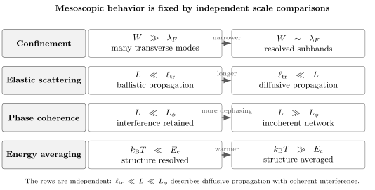
Mesoscopic classification is a ledger rather than one size axis. Confinement compares $W$ with $\lambda_F$; ballistic or diffusive propagation compares $L$ with $\ell_{\mathrm e}$ or $\ell_{\mathrm{tr}}$; coherence compares path length with $L_\phi$; and thermal resolution compares $k_{\mathrm B}T$ with the observable’s correlation or level scale $E_{\mathrm c}$. A conductor can be diffusive and phase coherent at the same time.

Nanoscopic is not synonymous with mesoscopic

Nanoscopic describes geometric size. Mesoscopic describes which physical information survives into an observable. A small metallic grain at high temperature may have a continuum-like spectrum and incoherent transport. A larger metal ring at millikelvin temperature may retain phase around its full circumference and display flux-periodic conductance.

Nor does mesoscopic mean “few particle.” A metal ring may contain an enormous Fermi sea. The distinctive quantum effect arises because electrons near the Fermi surface propagate coherently through a finite circuit and because the resulting interference pattern is not fully averaged away.

No single crossover is sharp

Most boundaries in the scale ledger are crossovers:

• transverse subbands become increasingly distinct as $W/\lambda_F$ decreases and disorder or temperature broadening weakens;
• transport evolves from ballistic to diffusive as $L/\ell_{\mathrm{tr}}$ grows;
• interference visibility decays continuously as path duration approaches the dephasing time;
• thermal convolution gradually smooths features narrower than $k_{\mathrm B}T$;
• localization develops when coherent multiple scattering becomes strong on the sample scale.

A paper or device description should state the hierarchy actually used rather than attach one regime label to the whole sample.

Microscopic Wavelength and Confinement

In a degenerate electron system, the states that control low-bias transport lie near the Fermi energy. Their characteristic wavelength is

$$\lambda_F = \frac{2\pi}{k_F}.$$

If a transverse width $W$ is much larger than $\lambda_F$, many modes fit and the boundary can often be represented by a smooth correction to bulk motion. If $W$ is comparable to $\lambda_F$, transverse motion is quantized. For a hard-wall strip,

$$k_{\perp,n} = \frac{n\pi}{W}, \qquad n=1,2,\ldots,$$

and a parabolic-band benchmark gives

$$E_n(k_\parallel) = \frac{\hbar^2}{2m^\ast} \left[ k_\parallel^2 + \left( \frac{n\pi}{W} \right)^2 \right].$$

The thresholds $E_n(0)$ are subband bottoms. Opening them one by one produces the channel-counting structure developed on Conductance Quantization.

Confinement and coherence are separate. A narrow wire can have resolved subbands but lose phase after a short distance. Conversely, a broad ring can support many modes while retaining coherent interference between its two arms.

Elastic Scattering and Momentum Relaxation

Let $\tau_{\mathrm e}$ be a single-particle elastic scattering time. A corresponding path length is

$$\ell_{\mathrm e} \sim v_F\tau_{\mathrm e}.$$

Elastic scattering changes momentum while preserving energy. For a static disorder potential it need not destroy phase coherence: the wave accumulates a well-defined, sample-specific phase along each multiply scattered path.

Transport is controlled more directly by the momentum-relaxation time $\tau_{\mathrm{tr}}$. In a schematic angular-scattering description,

$$\frac{1}{\tau_{\mathrm{tr}}} \propto \int d\Omega\, W(\theta) \left( 1-\cos\theta \right),$$

whereas the quantum or single-particle rate lacks the factor $1-\cos\theta$. Small-angle events can strongly broaden a single-particle state while relaxing net momentum only weakly. Thus

$$\ell_{\mathrm{tr}} = v_F\tau_{\mathrm{tr}}$$

can be substantially larger than $\ell_{\mathrm e}$ in a smooth disorder potential. Authors do not always use the symbols $\ell_{\mathrm e}$ and $\ell_{\mathrm{tr}}$ consistently, so the operative lifetime must be identified from context.

Ballistic propagation

A path is ballistic when its relevant length is shorter than the transport mean free path:

$$L \ll \ell_{\mathrm{tr}}.$$

Ballistic does not mean reflectionless. Boundaries, abrupt constrictions, mode mismatch, tunnel barriers, and contacts can all reflect carriers in an impurity-free device. The word only says that randomizing collisions in the interior are rare on the path of interest.

Diffusive propagation

When many elastic collisions occur but the motion remains extended,

$$\ell_{\mathrm{tr}} \ll L,$$

the coarse-grained probability density follows diffusion. For an isotropic $d$-dimensional parabolic band,

$$D \sim \frac{v_F^2\tau_{\mathrm{tr}}}{d} = \frac{v_F\ell_{\mathrm{tr}}}{d},$$

up to geometry and band-structure factors.

Diffusion is a statement about the disorder-averaged probability distribution. A particular electron amplitude still explores many coherent paths until dephasing occurs. That distinction is the origin of weak localization, flux-sensitive interference, and reproducible conductance fluctuations in a phase-coherent diffusive conductor.

Localization is not merely stronger diffusion

Coherent backscattering can eventually invalidate classical diffusion. In a localized regime, a typical transmission through length $L$ decreases approximately as

$$G_{\mathrm{typ}} \propto \exp \left( -\frac{L}{\xi_{\mathrm{loc}}} \right),$$

where $\xi_{\mathrm{loc}}$ is a localization length that depends on dimensionality, channel number, disorder, symmetry class, and interactions. A short sample can look metallic even when an asymptotically longer sample with the same microscopic disorder would localize. The dedicated disorder chapter owns the full scaling theory; the point here is that $L/\xi_{\mathrm{loc}}$ is another finite-size comparison.

Phase Coherence and Dephasing

Suppose an amplitude reaches the detector through paths $p$:

$$\mathcal A = \sum_p \mathcal A_p e^{i\varphi_p}.$$

The probability contains cross terms,

$$\lvert\mathcal A\rvert^2 = \sum_p \lvert\mathcal A_p\rvert^2 + \sum_{p\ne q} \mathcal A_p \mathcal A_q^\ast e^{i(\varphi_p-\varphi_q)}.$$

Mesoscopic interference is the survival of some of these cross terms in a measured quantity.

If $\tau_\phi$ is a dephasing time, a useful coherence length is

$$L_\phi \sim \begin{cases} v_F\tau_\phi, & \text{ballistic propagation}, \\[4pt] \sqrt{D\tau_\phi}, & \text{diffusive propagation}. \end{cases}$$

The numerical convention can differ by factors of order unity between fitting formulas. A quoted $L_\phi$ should therefore name the observable and model from which it was extracted.

What can cause dephasing?

Dephasing occurs when uncontrolled degrees of freedom acquire which-path information or randomize the relative phase. Mechanisms can include:

• electron–electron scattering with energy exchange;
• electron–phonon coupling;
• magnetic-impurity dynamics;
• electromagnetic noise and fluctuating charges;
• voltage-probe or detector backaction;
• escape into a reservoir;
• deliberately introduced time-dependent fields.

Static elastic disorder is not on this list by itself. It changes the phase pattern, but repeated measurements of the same frozen sample can reproduce that pattern.

Inelastic length and coherence length

Energy relaxation and phase relaxation are related but not identical. An inelastic event generally carries phase information into other degrees of freedom, but phase can also be randomized without a large net energy transfer. Depending on how the lifetimes are defined and which mechanism dominates, $\tau_\phi$ and $\tau_{\mathrm{in}}$ can differ parametrically; there is no universal equality or ordering to insert without a microscopic model. The relevant comparison is always with the duration and path separation of the measured interference process.

Thermal Averaging Is Not Dephasing

At finite temperature, a linear-response conductance samples an energy window through

$$G(T) = \int dE\, \left[ -\frac{\partial f(E)}{\partial E} \right] G(E,0),$$

where $f(E)$ is the Fermi–Dirac distribution. The kernel has width of order $k_{\mathrm B}T$. If $G(E,0)$ changes appreciably over an energy scale $E_{\mathrm c}$, then

$$k_{\mathrm B}T \gtrsim E_{\mathrm c}$$

smooths the structure even if every electron remains coherent while crossing the device.

This is ensemble averaging over occupied energies, not loss of phase along one trajectory. Temperature can do both: it broadens the energy window and changes microscopic dephasing rates. A careful analysis separates these effects.

The thermal time

$$\tau_T \sim \frac{\hbar}{k_{\mathrm B}T}$$

defines propagation lengths

$$L_T \sim \begin{cases} \dfrac{\hbar v_F}{k_{\mathrm B}T}, & \text{ballistic}, \\[10pt] \sqrt{ \dfrac{\hbar D}{k_{\mathrm B}T} }, & \text{diffusive}. \end{cases}$$

Factors such as $\pi$ or $2\pi$ appear in different correlation functions and conventions. The scaling and the stated definition matter more than an unexplained prefactor.

Traversal Time and Thouless Energy

Finite devices introduce a characteristic time for exploring the coherent region. In a ballistic segment,

$$\tau_{\mathrm{bal}} \sim \frac{L}{v_F}, \qquad E_{\mathrm{bal}} \sim \frac{\hbar v_F}{L}.$$

In a diffusive sample,

$$\tau_D \sim \frac{L^2}{D}, \qquad E_{\mathrm{Th}} \equiv \frac{\hbar D}{L^2}.$$

$E_{\mathrm{Th}}$ is the Thouless energy. It sets an order-of-magnitude spectral or transport correlation scale for diffusion across the sample. The relevant length may be the contact separation, ring circumference, or coherent block size rather than the largest lithographic dimension.

For a closed coherent region with mean single-particle level spacing $\Delta$, one also defines a Heisenberg time

$$\tau_H = \frac{h}{\Delta}.$$

Under standard diffusive-metal assumptions, the Thouless number obeys the order-of-magnitude relation

$$g_{\mathrm{Th}} \sim \frac{E_{\mathrm{Th}}}{\Delta}.$$

It is closely related, up to convention and geometry factors, to the dimensionless terminal conductance

$$g \equiv \frac{G}{e^2/h}.$$

This relation connects spectral sensitivity to boundary conditions with transport. It should not be used as an exact identity without specifying spin degeneracy, leads, boundary conditions, and the definition of $E_{\mathrm{Th}}$.

Open dwell time

An open cavity has another scale: the time $\tau_{\mathrm{dwell}}$ before a carrier escapes through the contacts. The associated resonance width is

$$\Gamma \sim \frac{\hbar}{\tau_{\mathrm{dwell}}}.$$

A geometrically tiny dot can have a long dwell time if its tunnel barriers are opaque. Thus openness is not determined by size alone. Whether individual resonances are resolved depends on the hierarchy among

$$\Delta, \quad \Gamma, \quad k_{\mathrm B}T, \quad e\lvert V\rvert, \quad E_{\mathrm{Th}}.$$

Contacts and Reservoirs Are Part of the System

Bulk transport is often phrased as a local constitutive law,

$$\mathbf j = \boldsymbol{\sigma}\mathbf E.$$

For a short coherent conductor, a unique local electric field or geometry-independent resistivity may not be the most useful description. The directly controlled quantities are reservoir electrochemical potentials and terminal currents.

For noninteracting coherent transport, the Landauer expression is

$$I = \frac{e}{h} \sum_n \int dE\, T_n(E) \left[ f_S(E)-f_D(E) \right].$$

In linear response at zero temperature,

$$G = \frac{e^2}{h} \sum_n T_n(E_F).$$

The full derivation and plateau diagnostics belong to Conductance Quantization. Here the conceptual lesson is that $G$ belongs to the device plus its contacts and measurement convention.

A perfect channel still has two-terminal resistance

One perfectly transmitted, spin-resolved channel has

$$G = \frac{e^2}{h}, \qquad R_{\mathrm{2t}} = \frac{h}{e^2}.$$

This does not imply dissipative scattering inside the channel. In the ideal Landauer picture, entropy production and equilibration occur in the reservoirs and contact regions. A four-terminal measurement can assign a different voltage drop because its probes alter which electrochemical potentials are compared.

Reservoirs do two jobs

Ideal reservoirs:

1. inject incoming modes with equilibrium occupations set by temperature and chemical potential;
2. absorb outgoing modes so thoroughly that their phase information is not returned to the coherent device.

The scattering matrix of the central elastic region can remain unitary even though the transport experiment is operationally irreversible after reservoir degrees of freedom are ignored.

Geometry changes the observable

Moving a voltage probe, opening a side lead, narrowing a constriction, or changing a ring arm can alter measured conductance without changing the nominal bulk material. In multiterminal form, currents are related to all reservoir potentials through transmission coefficients. The Onsager–Casimir relations constrain the magnetic-field reversal of that matrix, but they do not make every individual transmission coefficient even in $B$.

For a two-terminal conductor in linear response, microreversibility gives

$$G(B) = G(-B),$$

provided the equilibrium state and other time-reversal-odd parameters are reversed consistently. Multiterminal reciprocity instead exchanges source and detector indices.

Why Mesoscopic Observables Are Sample Specific

In a macroscopic disordered conductor, an observable averages over many coherence volumes, energy intervals, modes, and disorder regions. Microscopic interference corrections then become small relative to the mean response.

In a mesoscopic conductor, the number of independent coherent contributions can be modest. The exact impurity arrangement therefore produces a reproducible magnetofingerprint: a complicated but repeatable conductance pattern as magnetic field or gate voltage changes. Repeating a field sweep can reproduce the same pattern even though a nominally identical sample has a different one.

This is not experimental noise. Noise fluctuates between repeated measurements at fixed control parameters. A sample-specific interference pattern is reproducible until the impurity configuration, charge environment, or device state changes.

Universal conductance fluctuations

For a fully coherent diffusive conductor at low temperature, the root-mean-square fluctuation scale is of order

$$\operatorname{rms}\delta G \sim \frac{e^2}{h},$$

with coefficients determined by dimensionality, symmetry class, degeneracy, contacts, and geometry. “Universal” refers to the natural amplitude scale after the appropriate ensemble average, not to an identical trace in every sample.

Finite temperature and $L_\phi<L$ divide the device into partially independent regions and reduce the observed amplitude. Universal Conductance Fluctuations owns the correlation functions, symmetry crossover, geometry-dependent prefactors, and disorder-averaging logic.

Aharonov–Bohm rings

For two paths enclosing flux $\Phi$, the relative electromagnetic phase is

$$\Delta\varphi_{\mathrm{AB}} = \frac{e}{\hbar} \oint \mathbf A\cdot d\boldsymbol{\ell} = 2\pi \frac{\Phi}{h/e}.$$

If the effective enclosed area is $A_{\mathrm{eff}}$, the fundamental single-electron flux period corresponds to

$$\Delta B = \frac{h/e}{A_{\mathrm{eff}}}.$$

Seeing this period supports coherent paths around the ring, but a real trace can contain harmonics, time-reversed loops, spin phases, several occupied modes, changing effective area, and interaction effects. Aharonov–Bohm Effect owns the gauge-invariant phase itself.

A Device Taxonomy

Different geometries emphasize different comparisons:

Device	Confinement	Dominant finite-size physics	Typical observable
quantum well or two-dimensional gas	one confined direction	two-dimensional subbands and interface scattering	density, mobility, Hall response
quantum wire	two confined directions	one-dimensional subbands and enhanced interactions	conductance steps, one-dimensional density of states
quantum point contact	short tunable constriction	adiabatic mode opening and partition	plateaus and shot noise
quantum dot	confinement in all directions	level spacing, charging, dwell time	resonances and Coulomb diamonds
normal-metal or semiconductor ring	multiply connected path	flux-dependent relative phase	conductance oscillations and persistent currents
open cavity or electron billiard	boundary-controlled trajectories	dwell, escape, and chaotic scattering	conductance fluctuations and resonance statistics
hybrid normal–superconductor device	finite normal region plus pair potential	Andreev coherence and induced levels	subgap conductance and Josephson response

The same lithographic object can move between regimes as gates, temperature, field, density, or contact transparency change.

Worked Regime Diagnoses

A coherent diffusive ring

Consider a ring whose relevant path length is

$$L = 3.0\ \mu\mathrm m,$$

with

$$\ell_{\mathrm{tr}} = 0.30\ \mu\mathrm m, \qquad L_\phi = 6.0\ \mu\mathrm m.$$

Because

$$\ell_{\mathrm{tr}} \ll L \ll L_\phi,$$

the arms are diffusive but phase coherent. Let

$$D = 0.030\ \mathrm{m^2\,s^{-1}}.$$

Then

$$E_{\mathrm{Th}} = \frac{\hbar D}{L^2} \approx 2.2\ \mu\mathrm{eV}.$$

At $T=100\ \mathrm{mK}$,

$$k_{\mathrm B}T \approx 8.6\ \mu\mathrm{eV}, \qquad L_T \approx 1.5\ \mu\mathrm m.$$

Thermal averaging is therefore appreciable even though $L_\phi$ exceeds the circumference. The statements “coherent” and “thermally unresolved” can both be true.

If the effective enclosed area is $1.2\ \mu\mathrm m^2$, the expected $h/e$ field period is

$$\Delta B \approx 3.45\ \mathrm{mT}.$$

Agreement with this value is one part of the diagnosis; reproducibility, temperature dependence, harmonic content, and area calibration are also needed.

A ballistic constriction

Suppose a constriction has

$$W \sim \lambda_F, \qquad L_c \ll \ell_{\mathrm{tr}}, \qquad k_{\mathrm B}T \ll \Delta_\perp.$$

The first inequality resolves transverse modes, the second makes the constriction ballistic, and the third prevents thermal smearing of adjacent thresholds. Conductance plateaus additionally require sufficiently adiabatic contacts and transmission eigenvalues near unity. Narrow and ballistic are necessary parts of the story, not the whole explanation.

A small but long-lived dot

A $100\ \mathrm{nm}$ island may satisfy

$$L \ll \ell_{\mathrm{tr}}, L_\phi,$$

yet tunnel barriers can make

$$\tau_{\mathrm{dwell}} \gg \frac{L}{v_F}.$$

Its spectrum and linewidth are then controlled by confinement, charging, and escape rather than a simple ballistic flight. This is why Quantum Dots require both a geometry ledger and an energy-scale ledger.

Experimental Evidence Workflow

A defensible mesoscopic interpretation should answer the following questions.

Establish the geometric problem

State the contact separation, widths, thickness, ring area, dot volume, and barrier geometry relevant to the measurement. A scanning-electron micrograph alone does not give the electronic width because depletion and band bending shift the active boundary.

Estimate material scales

Infer carrier density, $k_F$, $\lambda_F$, $v_F$, mobility, and a transport mean free path using a model appropriate to the band structure and dimensionality. Do not insert a bulk effective mass into graphene or a multivalley semiconductor without checking the regime.

Separate coherence from mobility

Mobility mainly constrains momentum relaxation. Extract $L_\phi$ from an interference observable with a stated fitting model, such as weak-localization magnetoconductance, ring-harmonic decay, or fluctuation correlation scales. High mobility is not itself proof of long phase coherence.

State the energy window

Compare $k_{\mathrm B}T$, $e\lvert V\rvert$, modulation amplitude, detector bandwidth, and lifetime broadening with $\Delta$, $E_{\mathrm{Th}}$, subband spacing, or resonance width. Electron temperature can exceed the refrigerator temperature.

Include contacts and probes

Specify two-terminal versus multiterminal geometry, lead mode count, series resistance subtraction, contact transparency, impedance environment, and whether a charge detector or voltage probe adds dephasing.

Demand controlled variation

Vary magnetic field, gate voltage, temperature, bias, path length, or contact configuration. A coherent interpretation is strongest when periods, symmetry, correlation fields, amplitudes, and crossover scales move together as predicted.

Common Mistakes

• Defining mesoscopic physics by a fixed interval of metric size.
• Using nanoscopic, ballistic, coherent, and quantized as synonyms.
• Assuming elastic scattering destroys phase coherence.
• Assuming a high-mobility sample must have a long $L_\phi$.
• Treating thermal averaging and dephasing as the same mechanism.
• Writing $L_\phi=v_F\tau_\phi$ in a diffusive conductor.
• Confusing the elastic mean free path with the transport mean free path.
• Treating a two-terminal conductance as a bulk conductivity.
• Calling $h/e^2$ evidence for dissipation inside a perfect channel.
• Ignoring contact geometry and reservoir occupations.
• Calling a reproducible magnetofingerprint random measurement noise.
• Quoting a Thouless energy without stating which length and diffusion constant were used.
• Interpreting one flux period without checking effective area, harmonics, and alternative coherent loops.
• Inferring a universal fluctuation trace rather than a universal amplitude scale.

Exercises

1. Classify a narrow conductor

A wire has width $W=70\ \mathrm{nm}$, length $L=1.2\ \mu\mathrm m$, Fermi wavelength $\lambda_F=60\ \mathrm{nm}$, transport mean free path $\ell_{\mathrm{tr}}=0.25\ \mu\mathrm m$, and phase-coherence length $L_\phi=4.0\ \mu\mathrm m$. Classify confinement, propagation, and coherence separately.

Solution

Because $W$ is comparable to $\lambda_F$, transverse quantization should matter and only a modest number of modes fit. Since

$$\ell_{\mathrm{tr}} < L,$$

the longitudinal motion is diffusive rather than ballistic. Since

$$L < L_\phi,$$

the full wire can nevertheless remain phase coherent. The appropriate label is a transversely confined, coherent diffusive wire. None of the three adjectives implies either of the others.

2. Derive the diffusive thermal length

Starting from the thermal time $\tau_T\sim\hbar/(k_{\mathrm B}T)$ and the diffusion law $\langle r^2\rangle\sim D t$, derive the scaling of $L_T$.

Solution

During the thermal time, diffusion explores a distance

$$L_T^2 \sim D\tau_T.$$

Substituting $\tau_T$ gives

$$L_T \sim \sqrt{ \frac{\hbar D}{k_{\mathrm B}T} }.$$

The derivation fixes the scaling. Exact prefactors depend on whether the observable uses Matsubara frequencies, a particular diffusion mode, or a correlation-function convention.

3. Compare Thouless and thermal energies

A diffusive square has side $L=1.0\ \mu\mathrm m$ and diffusion constant $D=0.020\ \mathrm{m^2\,s^{-1}}$. Estimate $E_{\mathrm{Th}}$ and compare it with $k_{\mathrm B}T$ at $T=100\ \mathrm{mK}$.

Solution

The Thouless energy is

$$\begin{aligned} E_{\mathrm{Th}} &= \frac{\hbar D}{L^2} \\ &\approx \frac{ \left( 1.055\times10^{-34}\ \mathrm{J\,s} \right) \left( 0.020\ \mathrm{m^2\,s^{-1}} \right) }{ \left( 10^{-6}\ \mathrm m \right)^2 } \\ &\approx 2.11\times10^{-24}\ \mathrm J \\ &\approx 13.2\ \mu\mathrm{eV}. \end{aligned}$$

At $100\ \mathrm{mK}$,

$$k_{\mathrm B}T \approx 8.62\ \mu\mathrm{eV}.$$

The two scales are comparable, with $k_{\mathrm B}T<E_{\mathrm{Th}}$. Energy-dependent coherent structure on the Thouless scale is not strongly washed out, but this is a crossover rather than an asymptotically cold limit.

4. A perfect channel and finite resistance

Why can a perfectly transmitted spin-resolved channel have two-terminal resistance $h/e^2$ without dissipating energy inside the channel?

Solution

The terminal conductance compares current with the electrochemical-potential difference of two reservoirs. A single resolved incoming mode carries

$$G = \frac{e^2}{h}$$

when its transmission is one. The corresponding two-terminal resistance includes the conversion between equilibrium reservoir occupations and the directed channel population. In the ideal model, carriers propagate elastically through the channel; equilibration and entropy production occur when outgoing carriers enter macroscopic reservoirs. The finite terminal resistance is therefore not evidence for impurity scattering in the channel.

5. Flux period of a ring

A ring has effective area $A_{\mathrm{eff}}=0.80\ \mu\mathrm m^2$. What magnetic-field period corresponds to one single-electron flux quantum $h/e$?

Solution

Using

$$\frac{h}{e} \approx 4.136\times10^{-15}\ \mathrm{T\,m^2},$$

the period is

$$\begin{aligned} \Delta B &= \frac{h/e}{A_{\mathrm{eff}}} \\ &= \frac{ 4.136\times10^{-15}\ \mathrm{T\,m^2} }{ 0.80\times10^{-12}\ \mathrm{m^2} } \\ &\approx 5.17\ \mathrm{mT}. \end{aligned}$$

A measured period should be compared with the electronic rather than merely lithographic area, and harmonics should be identified separately.

6. Thermal averaging or dephasing?

An interference pattern loses contrast as temperature rises. Give two reasons why this observation alone does not identify the dephasing mechanism, and propose discriminating measurements.

Solution

First, the Fermi window broadens, so energy-dependent interference patterns can average out even if each carrier remains coherent. Second, the microscopic $\tau_\phi$ can itself decrease because electron–electron, electron–phonon, magnetic, or environmental processes become faster.

Useful controls include measuring finite-bias energy correlations to estimate $E_{\mathrm c}$, extracting $L_\phi(T)$ from a geometry-sensitive fit, comparing devices with different path lengths, tracking several ring harmonics, and independently measuring electron temperature. A contrast reduction consistent only with the thermal convolution need not imply a shorter pathwise coherence length.

7. Elastic disorder and repeatability

Why can a conductor with many impurity collisions show a reproducible conductance pattern, while changing the impurity configuration changes the pattern?

Solution

Static elastic impurities define a fixed set of scattering amplitudes and phases. If $L_\phi$ exceeds the relevant paths, repeated measurements sum the same coherent path amplitudes and reproduce the same magnetofingerprint. Rearranging impurities changes path phases and amplitudes, producing a different fingerprint. The first situation is coherent sample specificity; the second is a new disorder realization. Neither should be confused with time-dependent measurement noise.

8. Test a universal-fluctuation claim

Design a minimal evidence checklist for a claim of universal conductance fluctuations in a two-terminal device.

Solution

The conductance pattern should be reproducible on repeated magnetic-field sweeps and stable at fixed controls, distinguishing it from noise. Its two-terminal linear-response trace should satisfy $G(B)=G(-B)$ after offsets and hysteretic variables are controlled. The fluctuation amplitude should be compared with $e^2/h$ after removing a smooth background and stating degeneracy, geometry, and thermal averaging. Field and gate correlation scales should be consistent with a coherent area and an energy-correlation scale. Temperature or device-length dependence should reduce the amplitude as $L_\phi$ or $L_T$ becomes shorter. Thermal cycling or a controlled disorder rearrangement may change the detailed fingerprint while leaving its statistical scale comparable.

Connections

• Boltzmann Transport develops the bulk semiclassical distribution-function limit and collision integrals that mesoscopic finite geometry can invalidate.
• Reflection and Transmission Coefficients owns the elementary current-conserving scattering conventions behind channel transport.
• Mesoscopic Transport develops sequential tunneling, master equations, current noise, counting statistics, and reservoir-induced open dynamics.
• Quantum Coherence in Conductors develops phase-memory kernels, diffusive dephasing, weak-localization and fluctuation extractors, and the low-temperature saturation audit.
• Universal Conductance Fluctuations develops reproducible sample fingerprints, universal variance, correlation fields and energies, finite-coherence scaling, and ergodic averaging.
• Quantum Wires develops transverse confinement, subband occupation, one-dimensional threshold singularities, and the crossover among extended wires, point contacts, and dots.
• Conductance Quantization derives the Landauer channel contribution, contact resistance, degeneracy counting, and plateau diagnostics.
• Quantum Dots develops zero-dimensional confinement, addition energies, linewidths, spin filling, and optical variants.
• Coulomb Blockade develops the capacitance and tunnel-rate conditions for integer charging, Coulomb diamonds, and SET operation.
• Aharonov–Bohm Effect owns electromagnetic holonomy and gauge-invariant phase around a multiply connected path.
• Integer Quantum Hall Effect owns topological edge channels, plateau transport, disorder localization, and Hall-tensor conventions.
• Quantum Matter Conventions records charge, field, Fourier, response, and unit conventions used across solid-state pages.

Further Reading

• Y. Imry, Introduction to Mesoscopic Physics, 2nd ed., Oxford University Press (2002), doi:10.1093/oso/9780198507383.001.0001.
• S. Datta, Electronic Transport in Mesoscopic Systems, Cambridge University Press (1995), doi:10.1017/CBO9780511805776.
• E. Akkermans and G. Montambaux, Mesoscopic Physics of Electrons and Photons, Cambridge University Press (2007), doi:10.1017/CBO9780511618833.
• C. W. J. Beenakker and H. van Houten, “Quantum Transport in Semiconductor Nanostructures,” Solid State Physics 44, 1–228 (1991), doi:10.1016/S0081-1947(08)60091-0.

References

1. R. Landauer, “Spatial Variation of Currents and Fields Due to Localized Scatterers in Metallic Conduction,” IBM Journal of Research and Development 1, 223–231 (1957), doi:10.1147/rd.13.0223.
2. M. Büttiker, “Four-Terminal Phase-Coherent Conductance,” Physical Review Letters 57, 1761–1764 (1986), doi:10.1103/PhysRevLett.57.1761.
3. D. J. Thouless, “Maximum Metallic Resistance in Thin Wires,” Physical Review Letters 39, 1167–1169 (1977), doi:10.1103/PhysRevLett.39.1167.
4. P. A. Lee and T. V. Ramakrishnan, “Disordered Electronic Systems,” Reviews of Modern Physics 57, 287–337 (1985), doi:10.1103/RevModPhys.57.287.
5. R. A. Webb, S. Washburn, C. P. Umbach, and R. B. Laibowitz, “Observation of $h/e$ Aharonov–Bohm Oscillations in Normal-Metal Rings,” Physical Review Letters 54, 2696–2699 (1985), doi:10.1103/PhysRevLett.54.2696.
6. P. A. Lee and A. D. Stone, “Universal Conductance Fluctuations in Metals,” Physical Review Letters 55, 1622–1625 (1985), doi:10.1103/PhysRevLett.55.1622.
7. B. L. Altshuler, “Fluctuations in the Extrinsic Conductivity of Disordered Conductors,” JETP Letters 41, 648–651 (1985).
8. S. Washburn and R. A. Webb, “Aharonov–Bohm Effect in Normal Metal: Quantum Coherence and Transport,” Advances in Physics 35, 375–422 (1986), doi:10.1080/00018738600101911.
9. A. G. Aronov and Y. V. Sharvin, “Magnetic Flux Effects in Disordered Conductors,” Reviews of Modern Physics 59, 755–779 (1987), doi:10.1103/RevModPhys.59.755.
10. B. J. van Wees et al., “Quantized Conductance of Point Contacts in a Two-Dimensional Electron Gas,” Physical Review Letters 60, 848–850 (1988), doi:10.1103/PhysRevLett.60.848.
11. D. A. Wharam et al., “One-Dimensional Transport and the Quantisation of the Ballistic Resistance,” Journal of Physics C: Solid State Physics 21, L209–L214 (1988), doi:10.1088/0022-3719/21/8/002.
12. C. W. J. Beenakker, “Random-Matrix Theory of Quantum Transport,” Reviews of Modern Physics 69, 731–808 (1997), doi:10.1103/RevModPhys.69.731.