Quantum Point Contacts

A quantum point contact (QPC) is a short, gate-tunable constriction whose electronic width is comparable to the Fermi wavelength and whose length is shorter than the elastic mean free path. Wide reservoirs feed the constriction, transverse modes open one at a time, and the resulting transmission can be tuned continuously from pinch-off to several nearly transparent channels.

The word contact does not mean an ordinary metal–semiconductor interface. A semiconductor QPC is usually patterned inside one continuous two-dimensional electron gas (2DEG): negatively biased surface gates deplete carriers beneath and beside a narrow opening. Other platforms use etched graphene, oxide channels, nanowires, atomic contacts, or quantum Hall edge gates, but the operational question is the same: does a small number of coherent transmission eigenchannels control transport through a localized bottleneck?

This page owns the QPC as a device and detector: split-gate electrostatics, narrow-constriction geometry, local adiabatic modes, pinch-off and bias maps, beam-splitter operation, charge responsivity, bandwidth, and measurement backaction. Conductance Quantization owns the full Landauer derivation, degeneracy ledger, contact resistance, plateau metrology, saddle transmission formula, and shot-noise derivation. Quantum Wires owns extended one-dimensional subbands and density of states. Quantum Dots owns isolated-dot spectra, while Coulomb Blockade owns tunnel-junction thresholds and diamond-capacitance extraction. The formulas repeated here are used to explain how a QPC is tuned and measured, not to create a second canonical derivation.

Narrow Constrictions

Operational scale hierarchy

Let $W_{\mathrm{el}}$ be the electronic width at the bottleneck, $L_{\mathrm{QPC}}$ its longitudinal length, $\lambda_F$ the reservoir Fermi wavelength, $\ell_e$ the elastic mean free path, and $L_\phi$ the phase-coherence length. A clean few-mode QPC typically satisfies

$$W_{\mathrm{el}} \sim \lambda_F, \qquad L_{\mathrm{QPC}} \ll \ell_e, \qquad L_{\mathrm{QPC}} \lesssim L_\phi.$$

The first relation gives transverse quantization, the second suppresses random scattering inside the bottleneck, and the third permits a scattering-amplitude description across the device. A globally phase-coherent millimeter-scale circuit is not required for a conductance plateau. The reservoirs may dephase and thermalize carriers after they leave the constriction.

The transverse spacing $\Delta E_\perp$, temperature, source–drain bias, and lifetime broadening should obey

$$k_{\mathrm B}T, \ e\lvert V_{\mathrm{sd}}\rvert, \ \hbar/\tau_q \ll \Delta E_\perp$$

when sharply resolved zero-bias steps are desired. This is a resolution hierarchy, not a definition of ballisticity. A device can remain ballistic while thermal averaging hides its steps.

Split-gate electrostatics

In a GaAs/AlGaAs device, the 2DEG lies tens of nanometers below the surface. A sufficiently negative voltage on two metallic split gates raises the electron potential energy and depletes the 2DEG beneath them. Fringing fields also deplete part of the nominal gap, leaving a constriction narrower than the lithographic opening.

Consequently,

$$W_{\mathrm{el}} \neq W_{\mathrm{lith}}$$

in general. $W_{\mathrm{el}}$ depends on gate voltage, 2DEG depth, donor and dielectric geometry, screening, trapped charge, and neighboring electrodes. Quoting a gate separation as the electronic channel width without an electrostatic model or independent calibration is not reliable.

The gates chiefly control three device parameters:

Control	Physical effect	Experimental consequence
common-mode gate voltage	raises the bottleneck and narrows the channel	changes the number and transparency of modes
gate asymmetry	moves the channel laterally and changes transverse shape	tests disorder, edge roughness, and coupling to a nearby dot
source–drain bias	separates reservoir electrochemical potentials	maps subband thresholds and drives partition noise

Screening makes the self-consistent potential smoother than the metal edges. Near a clean bottleneck, a saddle is often a better local approximation than a rectangular aperture. At large negative voltage the constriction pinches off; at less negative voltage it opens into the parent 2DEG.

Fermi-wavelength estimate

For a spin-degenerate single-valley 2DEG,

$$n_{2\mathrm D} = \frac{k_F^2}{2\pi}, \qquad \lambda_F = \frac{2\pi}{k_F} = \sqrt{\frac{2\pi}{n_{2\mathrm D}}}.$$

At $n_{2\mathrm D}=2.0\times10^{15}\,\mathrm{m^{-2}}$,

$$\lambda_F \approx 56\,\mathrm{nm}.$$

A hard-wall aperture of width $W$ would support approximately

$$N_{\mathrm{orb}} \approx \left\lfloor \frac{k_FW}{\pi} \right\rfloor = \left\lfloor \frac{2W}{\lambda_F} \right\rfloor$$

occupied orbital modes. This estimate is useful for scale setting, but a real QPC has a smooth, gate-dependent profile and a longitudinal barrier. The observed step count is therefore a transmission measurement, not a direct ruler.

Point contact, wire, or dot?

Device	Longitudinal structure	Dominant spectrum	Typical gate trace
QPC	one short bottleneck	local transverse thresholds	steps separated by risers
quantum wire	extended narrow region	one-dimensional subbands over a long segment	subband features plus distributed scattering
quantum dot	island between two barriers	discrete addition spectrum	Coulomb peaks and diamonds

An unintended localized state can turn a QPC into a resonant constriction. Reproducible narrow peaks, Coulomb diamonds, strong hysteresis, or charge-switching lines are warnings that a pure saddle model is incomplete.

Local Adiabatic Modes

Let $x$ run along the constriction and $y$ across it. For an effective-mass Hamiltonian

$$H = -\frac{\hbar^2}{2m^\ast} \left( \partial_x^2+\partial_y^2 \right) +U(x,y),$$

define transverse eigenmodes at each $x$ by

$$\left[ -\frac{\hbar^2}{2m^\ast}\partial_y^2 +U(x,y) \right] \phi_n(y;x) = \varepsilon_n(x)\phi_n(y;x).$$

Expand the full wavefunction as

$$\Psi(x,y) = \sum_n \chi_n(x)\phi_n(y;x).$$

Projection onto mode $m$ gives

$$\begin{aligned} &\left[ -\frac{\hbar^2}{2m^\ast}\partial_x^2 +\varepsilon_m(x) \right]\chi_m(x) \\ &\quad -\frac{\hbar^2}{2m^\ast} \sum_n \left[ 2P_{mn}(x)\partial_x +Q_{mn}(x) \right]\chi_n(x) = E\chi_m(x), \end{aligned}$$

with derivative couplings

$$P_{mn} = \langle\phi_m\mid\partial_x\phi_n\rangle, \qquad Q_{mn} = \langle\phi_m\mid\partial_x^2\phi_n\rangle.$$

If the off-diagonal couplings are small, each local transverse mode propagates approximately independently through an effective one-dimensional potential $\varepsilon_n(x)$. A useful local criterion is

$$\hbar v_x \left| \langle\phi_m\mid\partial_x\phi_n\rangle \right| \ll \left| \varepsilon_m-\varepsilon_n \right| \qquad (m\neq n).$$

This is the spatial analogue of an adiabatic theorem: slow geometric variation suppresses mode conversion. It does not say that a mode crosses the bottleneck with unit probability. The longitudinal maximum of $\varepsilon_n(x)$ can still reflect it.

Define the $n$th threshold by

$$E_n^{\mathrm{top}} \equiv \max_x\varepsilon_n(x).$$

For chemical potential $\mu$ well above $E_n^{\mathrm{top}}$, the mode is open and can be nearly transparent. For $\mu$ well below it, the mode is evanescent near the bottleneck. The conductance riser occurs while the threshold passes through the reservoir energy window.

What makes a taper adiabatic?

For a width profile $W(x)$, the transverse eigenstates change on a geometric length

$$L_W \sim \left| \frac{W}{dW/dx} \right|.$$

The comparison is not simply $L_W\gg\lambda_F$. Near an avoided crossing of transverse modes, the relevant gap and symmetry matter. A symmetric constriction can forbid some couplings by parity, while disorder or lateral asymmetry can activate them. Numerical mode matching or a scattering-matrix calculation is needed when several thresholds approach one another or the gate shape is abrupt.

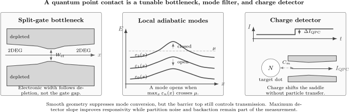
A QPC is a local bottleneck rather than a long wire. Split gates deplete a 2DEG and leave an electronic opening $W_{\mathrm{el}}$ smaller than the lithographic gap. Smooth transverse modes acquire $x$-dependent thresholds; modes below $\mu$ transmit while the next mode is tuned through its barrier top. A capacitively coupled dot shifts that saddle and produces a detector-current change $\Delta I_{\mathrm{QPC}}$ without requiring electron transfer between dot and detector.

Saddle Model and Gate Maps

Near the bottleneck, the standard separable saddle approximation is

$$U(x,y) = U_0 -\frac12m^\ast\omega_x^2x^2 +\frac12m^\ast\omega_y^2y^2.$$

$\hbar\omega_y$ sets the transverse spacing, while $\hbar\omega_x$ controls how rapidly each channel changes from closed to open. The orbital threshold energies are

$$E_n^{\mathrm{top}} = U_0 +\hbar\omega_y \left( n+\frac12 \right), \qquad n=0,1,2,\ldots$$

and the ideal transmission is

$$T_n(E) = \frac{1}{ 1+\exp\left[ -2\pi \dfrac{E-E_n^{\mathrm{top}}} {\hbar\omega_x} \right] }.$$

Thus $T_n=1/2$ exactly at the saddle threshold. A broader longitudinal barrier, corresponding to smaller $\omega_x$, produces a sharper energy transition. This exactly solvable local model is a calibration language, not proof that the full electrostatic potential is parabolic.

Over a limited gate range, a threshold can be linearized as

$$E_n^{\mathrm{top}}(V_g) \approx E_n^{\mathrm{top}}(V_g^{(0)}) -\alpha_ne \left( V_g-V_g^{(0)} \right),$$

where $\alpha_n$ is a gate lever arm in this convention. Finite-bias spectroscopy tracks where a threshold aligns with the source or drain electrochemical potential. The slopes of the resulting transconductance lines constrain $\alpha_n$ and bias division; their spacing estimates $\hbar\omega_y$.

The map is most informative when plotted as

$$\frac{\partial G}{\partial V_g} \quad\text{versus}\quad (V_g,V_{\mathrm{sd}}).$$

Bright threshold lines reveal risers that can be hard to locate on broad plateaus. Half-plateau structures may appear when a subband edge lies between the two reservoir potentials, but their value depends on bias symmetry and voltage drop. Conductance Quantization gives the full finite-bias interpretation and warns against assigning a universal half-step without that ledger.

Conductance Quantization in a QPC

If the channel index $a$ includes every resolved spin, valley, and orbital state, linear response gives

$$G = \frac{e^2}{h} \sum_a \int dE\, \left( -\frac{\partial f}{\partial E} \right) T_a(E).$$

At zero temperature,

$$G = \frac{e^2}{h} \sum_a T_a(\mu).$$

An ideal spin-degenerate QPC therefore approaches plateaus at $2Ne^2/h$. The plateau is a statement about nearly binary transmission eigenvalues, not about an integer number of electrons stored in the constriction. Dissipation occurs in the reservoirs where the nonequilibrium populations relax, even if the bottleneck itself is elastic.

Three distinct smoothings should not be conflated:

1. Intrinsic saddle rounding: $T_n(E)$ changes over an energy scale set by $\hbar\omega_x$.
2. Thermal rounding: the derivative $-\partial f/\partial E$ averages transmission over a window of order a few $k_{\mathrm B}T$.
3. Device inhomogeneity: disorder, gate noise, charge rearrangement, or series resistance distorts the trace.

Plateau alignment alone cannot determine the individual $T_a$. Different transmission sets can have the same sum. Shot noise, nonlinear spectroscopy, magnetic-field splitting, and source–drain asymmetry provide independent information.

Common nonideal structures

Resonances. Multiple reflections between the QPC and another scatterer create Fabry–Pérot-like structure. A localized state near the saddle can instead produce resonant or Fano line shapes.

The 0.7 structure. A shoulder near $0.7(2e^2/h)$ often appears below the first spin-degenerate plateau. Its evolution with temperature, density, source–drain bias, and magnetic field points to interaction and spin physics, but no single elementary saddle correction accounts for all observations. Its canonical diagnostic discussion remains at Conductance Quantization.

Series resistance. Leads, ohmic contacts, filters, and wiring add resistance. Choosing a subtraction solely to force integer plateaus is circular; it should be independently calibrated.

Charge switching. Telegraph jumps and hysteresis can come from traps rather than the intended channel. They also contaminate QPC charge detection unless target-dot transitions are distinguished by gate slopes, timing, or compensated sweeps.

Shot Noise

At low temperature and frequency, a biased coherent QPC produces partition noise

$$S_I = \frac{2e^3\lvert V_{\mathrm{sd}}\rvert}{h} \sum_a T_a(1-T_a)$$

when the transmissions are nearly energy independent over the bias window. Relative to the Poisson value $2e\lvert I\rvert$, the Fano factor is

$$F = \frac{ \sum_aT_a(1-T_a) }{ \sum_aT_a }.$$

Closed channels carry no current, and perfectly open channels are noiseless in this partition contribution. Noise is largest on a riser, where at least one $T_a$ is intermediate, and suppressed on a clean plateau. This makes shot noise a channel diagnostic that conductance alone cannot replace.

For energy-independent transmissions at a common temperature, the zero-frequency interpolation is

$$\begin{aligned} S_I(V,T) ={}& 4k_{\mathrm B}T \frac{e^2}{h} \sum_aT_a^2 \\ &+ 2e\lvert V\rvert \coth\left( \frac{e\lvert V\rvert}{2k_{\mathrm B}T} \right) \frac{e^2}{h} \sum_aT_a(1-T_a). \end{aligned}$$

As $V\to0$, the two terms combine to $4k_{\mathrm B}TG$. Comparing measured noise with this crossover requires a declared one-sided or two-sided spectral-density convention, amplifier gain and bandwidth, electron temperature, and subtraction of background voltage and current noise.

The detector role below creates an important tension: a plateau has little partition noise but also little charge responsivity because $\partial G/\partial V_g\approx0$. A riser is sensitive precisely because its transmission is changing, but it carries detector noise and stronger backaction.

QPCs as Charge Detectors

Place a quantum dot near, but electrically isolated from, a QPC. A change in dot charge shifts the electrostatic potential of the bottleneck through mutual capacitance. If the QPC is biased on a conductance riser, that shift changes its current.

Let one added electron shift the effective QPC gate voltage by $\beta$. In linear response,

$$\Delta I_{\mathrm{QPC}} \approx V_{\mathrm d} \frac{\partial G}{\partial V_g} \beta,$$

where $V_{\mathrm d}$ is the detector bias. The sign depends on gate and carrier conventions. The magnitude increases with capacitive coupling, detector bias, and transconductance.

This is charge sensing, not necessarily transport through the target. The dot can be nearly isolated, with current far below a direct ammeter’s resolution, while a nearby QPC records its occupation. A two-dimensional charge-stability diagram uses detector transconductance to reveal dot–lead and interdot charge transitions.

Charge sensitivity and integration time

Define current responsivity to target charge by

$$\mathcal R_q \equiv \left| \frac{\partial I_{\mathrm{QPC}}}{\partial q} \right|.$$

For a total one-sided detector-current noise spectral density $S_I^{(1)}$, the input-referred charge sensitivity is

$$s_q^{1/2} = \frac{ \sqrt{S_I^{(1)}} }{ \mathcal R_q },$$

with units $\mathrm{C}/\sqrt{\mathrm{Hz}}$, often reported as $e/\sqrt{\mathrm{Hz}}$. If white noise is averaged with an ideal rectangular window of duration $\tau$, the variance of the averaged current is

$$\sigma_{\bar I}^2 = \frac{S_I^{(1)}}{2\tau}.$$

Two charge states separated by $\Delta I$ therefore have squared signal-to-noise ratio

$$\mathrm{SNR}^2 = \frac{ 2(\Delta I)^2\tau }{ S_I^{(1)} }$$

under this convention. Real filters correlate samples and modify the numerical factor; calibration should use the measured transfer function rather than nominal bandwidth alone.

Time-resolved tunneling

If the measurement bandwidth exceeds the target tunnel rates, individual loading and unloading events appear as telegraph steps. Their dwell-time distributions determine tunnel rates. Counting events gives currents too small for direct dc measurement and provides full counting statistics.

Finite bandwidth biases the result. Closely spaced opposite transitions can merge into one unresolved excursion, making measured rates too small and suppressing high-order cumulants. A credible event-counting analysis reports:

• detector transfer function and sampling rate;
• threshold or hidden-state inference method;
• state-dependent noise and drift;
• dead-time or missed-event correction;
• a comparison between inferred and directly measurable current where possible.

Spin readout is spin-to-charge conversion

A QPC is primarily an electrometer. In energy-selective spin readout, only one spin state can tunnel during the read window; in Pauli-blockade readout, spin controls whether an interdot charge transition is allowed. The QPC then distinguishes the resulting charge histories.

Calling this a direct spin measurement hides the conversion stage. Readout fidelity factors into initialization error, spin-to-charge conversion error, relaxation during the window, detector overlap, and thresholding error. Spin Qubits owns the full control and readout protocol.

Radio-frequency operation

Embedding a QPC in an impedance-matching resonator converts charge-dependent conductance into a reflected amplitude or phase. Radio-frequency readout can move the signal away from low-frequency $1/f$ noise and raise bandwidth, but it adds resonator ring-up, impedance matching, amplifier noise, and microwave-induced backaction. The quoted bandwidth must distinguish the resonator linewidth, digital-filter bandwidth, and demonstrated single-event bandwidth.

Detector Backaction

A detector that acquires information must couple to the target. “Noninvasive” means no particle exchange through the sensing circuit, not zero disturbance.

QPC backaction includes:

1. Static electrostatic loading. Detector gate and bias voltages shift dot levels and tunnel barriers. Compensating gate sweeps can separate this deterministic cross-capacitance from stochastic backaction.
2. Measurement-induced dephasing. Scattered detector electrons become entangled with different target charge states. If their outgoing states are distinguishable, target coherence is reduced even when the detector record is ignored.
3. Nonequilibrium electrical noise. QPC charge and current fluctuations drive target-potential fluctuations. Frequency-resolved noise matters when a transition requires energy $\hbar\omega$.
4. Photon or phonon emission. A biased constriction can excite a nearby dot or double dot through electromagnetic or lattice coupling.
5. Heating. Detector power raises local electron or lattice temperature and changes target rates.

Increasing $\lvert V_{\mathrm d}\rvert$ generally improves $\Delta I$ only while the detector response remains linear. It also increases partition noise, available emission energy, and dissipated power. Maximum signal is therefore not the same as optimum fidelity.

An ideal quantum-limited detector converts all target-dependent changes in its scattering state into accessible information. A current measurement usually senses transmission changes but may discard target-dependent scattering phases. That unobserved information can dephase the target without improving the recorded signal. Measurement rate and dephasing rate should therefore be compared under one explicit noise convention rather than assumed equal.

The classic which-path experiment used a QPC to distinguish electron paths through a neighboring interferometer. Increasing detector sensitivity reduced interference visibility. This is not a technical accident: the same coupling that makes the paths distinguishable carries away their relative phase information.

QPCs as Beam Splitters and Local Probes

A partially transmitting QPC is an electronic beam splitter. In quantum Hall devices it mixes incoming edge channels and supports partition-noise, interferometry, and collision experiments. Chirality changes the terminal bookkeeping, while the local transmission language remains useful. Integer Quantum Hall Effect owns the bulk–edge and plateau mechanism.

QPCs also act as tunable tunnel barriers for quantum dots, injectors into ballistic cavities, spectrometers of one-dimensional subbands, and local thermoelectric filters. In each role, a single gate voltage can simultaneously change barrier height, width, density, and capacitive coupling. Interpreting it as a pure transmission knob is an approximation to test, not an experimental fact.

Evidence and Analysis Workflow

A convincing QPC characterization closes several loops:

1. Locate the regime. Estimate $\lambda_F$, $\ell_e$, $L_\phi$, $\Delta E_\perp$, $k_{\mathrm B}T$, and bias energy.
2. Map the gates. Record conductance and transconductance versus common-mode and asymmetric gate voltages; identify pinch-off, stable plateaus, hysteresis, and charge jumps.
3. Calibrate energy. Use finite-bias spectroscopy or an independent lever arm rather than converting gate voltage to energy by geometry alone.
4. Check channel information. Compare conductance, shot noise, magnetic splitting, and nonlinear response where the claim needs individual transmissions.
5. Audit contacts. Determine series resistance and terminal configuration independently.
6. For sensing, calibrate coupling. Measure $\Delta I$, total noise, transfer function, bandwidth, event fidelity, and detector-induced rate changes versus bias.
7. Test alternatives. Shift the channel laterally, warm the device, change sweep direction, and compare cooldowns to expose localized states and charge traps.

Claim	Supporting evidence	Main alternative
ballistic few-mode constriction	stable steps, bias subbands, $\ell_e\gg L_{\mathrm{QPC}}$	accidental resonances or series-resistance alignment
nearly open channel	conductance near a plateau and suppressed partition noise	several partial channels with the same total conductance
target charge transition	calibrated detector step with correct stability-diagram slope	trap switching or direct gate pickup
time-resolved single-electron event	two-state trace, exponential dwell statistics, bandwidth correction	thresholded amplifier noise
spin readout	validated spin-to-charge protocol plus charge discrimination	charge sensing without spin selectivity
weak backaction	target rates and coherence unchanged over detector operating range	unresolved heating or high-frequency emission

Common Mistakes

Equating gate gap with electronic width

Fringing depletion and screening make $W_{\mathrm{el}}$ gate- and material-dependent.

Calling every narrow channel a QPC

A long wire, tunnel junction, unintended dot, or diffusive neck can all be narrow without realizing an adiabatic ballistic point contact.

Treating adiabatic as perfectly transmitting

Adiabaticity suppresses mode conversion. A local threshold can still reflect the same mode.

Inferring channels from conductance alone

$G$ measures $\sum_aT_a$. Shot noise or another independent observable is needed to constrain the distribution of $T_a$.

Calling plateau noise zero

Partition noise vanishes for ideal binary transmissions, but thermal, amplifier, charge-trap, and environmental noise remain.

Operating a detector at maximum slope without a backaction audit

The riser improves responsivity but also carries partition noise and often stronger target disturbance.

Calling QPC spin readout direct

The detector senses charge after an energy-selective or Pauli-blockade conversion.

Ignoring missed events

Finite detector bandwidth removes short dwell intervals and biases inferred rates and counting statistics.

Exercises

1. Count hard-wall modes

A spin-degenerate 2DEG has density $n_{2\mathrm D}=2.0\times10^{15}\,\mathrm{m^{-2}}$. Estimate $\lambda_F$ and the number of occupied orbital modes in a hard-wall constriction with $W=120\,\mathrm{nm}$.

Solution

For one valley and two spin states,

$$\lambda_F = \sqrt{\frac{2\pi}{n_{2\mathrm D}}} \approx 56\,\mathrm{nm}.$$

The orbital count is

$$N_{\mathrm{orb}} \approx \left\lfloor \frac{2W}{\lambda_F} \right\rfloor = \left\lfloor \frac{240}{56} \right\rfloor = 4.$$

If all four orbital modes are nearly open and spin remains unresolved, the ideal conductance is $8e^2/h$. A smooth saddle and gate depletion can change the threshold positions, so this is a scale estimate rather than a plateau prediction.

2. Estimate a transverse spacing

Use an infinite square well of width $W=80\,\mathrm{nm}$ and GaAs mass $m^\ast=0.067m_e$. Estimate $E_2-E_1$.

Solution

For

$$E_n = \frac{\hbar^2\pi^2n^2}{2m^\ast W^2},$$

the first spacing is

$$E_2-E_1 = \frac{3\hbar^2\pi^2}{2m^\ast W^2} \approx 2.6\,\mathrm{meV}.$$

This corresponds to about $30\,\mathrm K$ as an energy divided by $k_{\mathrm B}$, although clean plateau resolution also depends on longitudinal rounding and disorder.

3. Test a saddle threshold

For one mode, let $\hbar\omega_x=0.40\,\mathrm{meV}$ and $E-E_n^{\mathrm{top}}=0.20\,\mathrm{meV}$. Find $T_n$. What is $T_n$ at threshold?

Solution

The exponent is

$$-2\pi \frac{E-E_n^{\mathrm{top}}}{\hbar\omega_x} = -\pi.$$

Hence

$$T_n = \frac{1}{1+e^{-\pi}} \approx 0.959.$$

At $E=E_n^{\mathrm{top}}$, the exponent vanishes and $T_n=1/2$.

4. Conductance does not fix shot noise

Two nondegenerate channels have transmissions $T_1=1$ and $T_2=0.4$. Find $G$ and $F$. Compare with two channels having $T_1=T_2=0.7$, which have the same conductance.

Solution

For the first set,

$$G = \frac{e^2}{h}(1+0.4) = 1.4\frac{e^2}{h},$$

and

$$F = \frac{0+0.4(0.6)}{1.4} \approx 0.171.$$

For $(0.7,0.7)$,

$$F = \frac{2(0.7)(0.3)}{1.4} = 0.300.$$

The equal conductances hide different transmission distributions; partition noise separates them.

5. Compare thermal and subband scales

A QPC has $\Delta E_\perp=1.5\,\mathrm{meV}$. Compare $k_{\mathrm B}T$ with this spacing at $T=100\,\mathrm{mK}$ and $T=10\,\mathrm K$.

Solution

Using $k_{\mathrm B}=0.08617\,\mathrm{meV/K}$,

$$k_{\mathrm B}T \approx 0.0086\,\mathrm{meV}$$

at $100\,\mathrm{mK}$, far below the spacing. At $10\,\mathrm K$,

$$k_{\mathrm B}T \approx 0.862\,\mathrm{meV},$$

which is comparable enough that the Fermi window strongly rounds neighboring risers. The exact visibility also depends on $\hbar\omega_x$ and broadening.

6. Detector response

A QPC is biased at $V_{\mathrm d}=200\,\mu\mathrm V$. Its transconductance is

$$\frac{\partial G}{\partial V_g} = 0.08 \frac{e^2/h}{\mathrm{mV}},$$

and one electron on a nearby dot produces an effective gate shift $\beta=0.15\,\mathrm{mV}$. Estimate $\Delta I_{\mathrm{QPC}}$.

Solution

The conductance shift is

$$\Delta G = 0.08(0.15)\frac{e^2}{h} = 0.012\frac{e^2}{h}.$$

Since $e^2/h\approx38.7\,\mu\mathrm S$,

$$\Delta G \approx 0.465\,\mu\mathrm S.$$

Therefore

$$\Delta I = V_{\mathrm d}\Delta G \approx (200\,\mu\mathrm V) (0.465\,\mu\mathrm S) \approx 93\,\mathrm{pA}.$$

This estimate assumes linear detector response and ignores bias-induced changes in the target.

7. Integration time from charge sensitivity

A detector has one-sided current-noise amplitude $20\,\mathrm{fA}/\sqrt{\mathrm{Hz}}$ and a one-electron signal $\Delta I=100\,\mathrm{fA}$. Under the rectangular-window convention above, how long is required for $\mathrm{SNR}=5$?

Solution

The spectral density is

$$S_I^{(1)} = \left( 20\,\mathrm{fA}/\sqrt{\mathrm{Hz}} \right)^2.$$

From

$$\mathrm{SNR}^2 = \frac{2(\Delta I)^2\tau}{S_I^{(1)}},$$

we obtain

$$\tau = \frac{ \mathrm{SNR}^2S_I^{(1)} }{ 2(\Delta I)^2 } = \frac{25}{2} \left( \frac{20}{100} \right)^2 \mathrm s = 0.50\,\mathrm s.$$

A real filter can require a different time, so the measured transfer function belongs in a fidelity budget.

8. Diagnose a resonant constriction

A nominal QPC shows narrow conductance peaks, closed diamonds in finite-bias spectroscopy, and strong sensitivity to sweep direction. Why is a pure adiabatic saddle interpretation doubtful, and what checks would you perform?

Solution

Closed diamonds indicate an isolated addition spectrum rather than only local subband thresholds. Narrow peaks and hysteresis suggest an unintended quantum dot or charge trap near the bottleneck. Useful checks include reversing the sweep, changing temperature, shifting the channel with asymmetric gate voltages, comparing cooldowns, mapping neighboring gates, and testing for telegraph noise. A model with one or more localized states coupled to leads is more appropriate if the charging signatures persist.

Connections

• Conductance Quantization owns the Landauer derivation, channel and degeneracy counting, finite-temperature and finite-bias plateaus, contact resistance, saddle transmission, and shot-noise derivation.
• Quantum Wires develops transverse subbands, local modes, Fermi points, and the one-dimensional density of states before a short bottleneck is introduced.
• Two-Dimensional Electron Gases supplies the parent density, Fermi scales, disorder lifetimes, interface confinement, and Hall-readiness ledger.
• Quantum Dots owns confinement, microscopic addition spectra, shell filling, and spin spectroscopy in the target devices that QPCs often sense.
• Coulomb Blockade explains when charge sectors remain sharp, how diamond edges encode capacitances, and why a nearby detector can resolve individual loading events.
• Single-Electron Devices compares SET and QPC electrometry and carries calibrated charge records into pumps, turnstiles, and quantized-current metrology.
• Quantum Coherence in Conductors distinguishes elastic phase-preserving scattering from dephasing and gives coherence-length diagnostics.
• Aharonov–Bohm Rings uses tunable transmissions as beam splitters and shows how detector coupling can reduce ring visibility.
• Mesoscopic Transport develops reservoir master equations, counting statistics, detector records, and open-system backaction.
• Spin Qubits owns spin-to-charge conversion, single-shot readout, relaxation, and fidelity accounting.
• Nanostructures for Quantum Technology places QPC control and electrometry inside an architecture ledger for bandwidth, crosstalk, calibration, wiring, and evidence.
• Integer Quantum Hall Effect places QPC beam splitters within chiral edge transport and multi-terminal Hall geometry.
• Reflection and Transmission Coefficients defines current-normalized elementary scattering probabilities.
• Conventions for Quantum Matter fixes charge, current, spectral-density, and response conventions.

Further Reading

• C. W. J. Beenakker and H. van Houten, “Quantum Transport in Semiconductor Nanostructures,” Solid State Physics 44, 1–228 (1991), doi:10.1016/S0081-1947(08)60091-0.
• Y. M. Blanter and M. Büttiker, “Shot Noise in Mesoscopic Conductors,” Physics Reports 336, 1–166 (2000), doi:10.1016/S0370-1573(99)00123-4.
• T. Ihn, Semiconductor Nanostructures: Quantum States and Electronic Transport, Oxford University Press, 2010.
• A. A. Clerk, M. H. Devoret, S. M. Girvin, F. Marquardt, and R. J. Schoelkopf, “Introduction to Quantum Noise, Measurement, and Amplification,” Reviews of Modern Physics 82, 1155–1208 (2010), doi:10.1103/RevModPhys.82.1155.

References

1. B. J. van Wees et al., “Quantized Conductance of Point Contacts in a Two-Dimensional Electron Gas,” Physical Review Letters 60, 848–850 (1988), doi:10.1103/PhysRevLett.60.848.
2. D. A. Wharam et al., “One-Dimensional Transport and the Quantisation of the Ballistic Resistance,” Journal of Physics C: Solid State Physics 21, L209–L214 (1988), doi:10.1088/0022-3719/21/8/002.
3. A. Szafer and A. D. Stone, “Theory of Quantum Conduction through a Constriction,” Physical Review Letters 62, 300–303 (1989), doi:10.1103/PhysRevLett.62.300.
4. M. Büttiker, “Quantized Transmission of a Saddle-Point Constriction,” Physical Review B 41, 7906–7909 (1990), doi:10.1103/PhysRevB.41.7906.
5. J. H. Davies, I. A. Larkin, and E. V. Sukhorukov, “Modeling the Patterned Two-Dimensional Electron Gas: Electrostatics,” Journal of Applied Physics 77, 4504–4512 (1995), doi:10.1063/1.359446.
6. K. J. Thomas et al., “Possible Spin Polarization in a One-Dimensional Electron Gas,” Physical Review Letters 77, 135–138 (1996), doi:10.1103/PhysRevLett.77.135.
7. G. B. Lesovik, “Excess Quantum Noise in 2D Ballistic Point Contacts,” JETP Letters 49, 592–594 (1989).
8. M. Reznikov, M. Heiblum, H. Shtrikman, and D. Mahalu, “Quantum Shot Noise,” Physical Review Letters 75, 3340–3343 (1995), doi:10.1103/PhysRevLett.75.3340.
9. A. Kumar, L. Saminadayar, D. C. Glattli, Y. Jin, and B. Etienne, “Experimental Test of the Quantum Shot Noise Reduction Theory,” Physical Review Letters 76, 2778–2781 (1996), doi:10.1103/PhysRevLett.76.2778.
10. M. Field, C. G. Smith, M. Pepper, D. A. Ritchie, J. E. F. Frost, G. A. C. Jones, and D. G. Hasko, “Measurements of Coulomb Blockade with a Noninvasive Voltage Probe,” Physical Review Letters 70, 1311–1314 (1993), doi:10.1103/PhysRevLett.70.1311.
11. S. A. Gurvitz, “Measurements with a Noninvasive Detector and Dephasing Mechanism,” Physical Review B 56, 15215–15223 (1997), doi:10.1103/PhysRevB.56.15215.
12. E. Buks, R. Schuster, M. Heiblum, D. Mahalu, and V. Umansky, “Dephasing in Electron Interference by a ‘Which-Path’ Detector,” Nature 391, 871–874 (1998), doi:10.1038/36057.
13. W. Lu, Z. Ji, L. Pfeiffer, K. W. West, and A. J. Rimberg, “Real-Time Detection of Electron Tunnelling in a Quantum Dot,” Nature 423, 422–425 (2003), doi:10.1038/nature01642.
14. J. M. Elzerman et al., “Single-Shot Read-Out of an Individual Electron Spin in a Quantum Dot,” Nature 430, 431–435 (2004), doi:10.1038/nature02693.
15. S. Gustavsson et al., “Counting Statistics of Single-Electron Transport in a Quantum Dot,” Physical Review Letters 96, 076605 (2006), doi:10.1103/PhysRevLett.96.076605.