Boltzmann Transport

Boltzmann transport is the semiclassical kinetic theory of how quasiparticle occupations move through phase space and are redistributed by collisions. Its central object is not a single drift velocity but a band- and momentum-resolved distribution

$$f_n(\mathbf r,\mathbf k,t).$$

For fermionic Bloch quasiparticles, $0\le f_n\le1$. The Boltzmann equation balances streaming under the band dynamics against a collision integral:

$$\frac{\partial f_n}{\partial t} + \dot{\mathbf r}\cdot \boldsymbol\nabla_{\mathbf r}f_n + \dot{\mathbf k}\cdot \boldsymbol\nabla_{\mathbf k}f_n = \mathcal I_n[f].$$

This framework improves on a one-number Drude model in three ways:

1. it resolves the Fermi-surface or band-state dependence of velocity and scattering;
2. it distinguishes scattering out of a state from scattering back into the current-carrying distribution;
3. it treats electrical, thermal, thermoelectric, spatial, and magnetic driving within one kinetic equation.

The improvement comes with a sharper burden of proof. A useful Boltzmann calculation must identify its quasiparticles, derive or justify its transition rates, preserve the relevant conservation laws, and establish a regime in which coherent quantum evolution can be reduced to a distribution function.

This page owns semiclassical electronic Boltzmann transport in materials. Drude Theory owns the single-relaxation-time benchmark and its optical response. Transport Coefficients Preview owns general transport limits and hydrodynamic classification, while Kubo Formula owns the exact equilibrium linear-response construction.

Required background. Band Theory Overview supplies the Bloch-band energies, state labels, occupations, and velocities used in $f_n(\mathbf k)$ without rederivation.

Semiclassical Dynamics of Bloch Electrons owns the collisionless trajectory of one packet and the isolated-band tests that supply this equation’s streaming kernel. This page retains distributions, collision operators, lifetimes, and transport coefficients; one packet trajectory is not yet a conductivity.

Helpful background. Drude Theory supplies the one-time benchmark; Fermi Surface and Density of States support metallic phase-space and state counting; Phonons supplies lattice-scattering inputs; and Transport Coefficients Preview supplies general limit, constitutive, and Onsager taxonomy.

Distribution Functions and State Counting

Let $n$ label a band and let $\mathbf k$ lie in the first Brillouin zone. Spin, valley, and other discrete labels may be included in $n$ or supplied as explicit degeneracy factors, but never both.

For a $d$-dimensional bulk system, the carrier density is

$$n_{\mathrm c} = \sum_n \int_{\mathrm{BZ}} \frac{d^dk}{(2\pi)^d} f_n(\mathbf k).$$

This normalization gives density per $d$-dimensional volume. A two-dimensional sheet density and a three-dimensional volume density are not interchangeable.

At local equilibrium,

$$f_n^0(\mathbf r,\mathbf k) = \frac{1}{ \exp\left[ \dfrac{ \varepsilon_n(\mathbf k)-\mu(\mathbf r) }{ k_{\mathrm B}T(\mathbf r) } \right] +1 }.$$

The derivative

$$- \frac{\partial f^0} {\partial\varepsilon} = \frac{1}{ 4k_{\mathrm B}T } \operatorname{sech}^2 \left[ \frac{ \varepsilon-\mu }{ 2k_{\mathrm B}T } \right]$$

is positive, integrates to one over an unrestricted energy axis, and selects a window of width of order $k_{\mathrm B}T$ around $\mu$.

Charge and heat currents

For carriers with signed charge $q$, the uniform transport currents are

$$\mathbf j = q \sum_n \int_{\mathrm{BZ}} \frac{d^dk}{(2\pi)^d} \mathbf v_n(\mathbf k) f_n(\mathbf k),$$ $$\mathbf j_Q = \sum_n \int_{\mathrm{BZ}} \frac{d^dk}{(2\pi)^d} \left[ \varepsilon_n(\mathbf k)-\mu \right] \mathbf v_n(\mathbf k) f_n(\mathbf k).$$

The heat current transports energy relative to the electrochemical work per particle. In transverse thermal response, equilibrium magnetization currents must also be separated from transport currents; that refinement is outside the zero-field longitudinal derivation below.

Semiclassical Streaming

For an isolated nondegenerate band without Berry-curvature corrections,

$$\dot{\mathbf r} = \mathbf v_n(\mathbf k) = \frac{1}{\hbar} \boldsymbol\nabla_{\mathbf k} \varepsilon_n(\mathbf k),$$

and

$$\hbar\dot{\mathbf k} = q \left[ \mathbf E + \dot{\mathbf r} \times \mathbf B \right].$$

The wave packet moves with band velocity, while the Lorentz force changes crystal momentum. These equations assume that the external fields vary slowly across the packet and do not induce appreciable interband transitions.

Substitution into the kinetic equation gives

$$\begin{aligned} \frac{\partial f_n}{\partial t} &+ \mathbf v_n\cdot \boldsymbol\nabla_{\mathbf r}f_n \\ &+ \frac{q}{\hbar} \left( \mathbf E + \mathbf v_n\times\mathbf B \right) \cdot \boldsymbol\nabla_{\mathbf k}f_n = \mathcal I_n[f]. \end{aligned}$$

Berry curvature can add an anomalous velocity and modify the phase-space measure. Strong fields can produce Landau quantization or magnetic breakdown. Those effects are not corrections to be inserted selectively: the equations of motion, density of states, orbital moment, and current must be updated consistently.

Collision Integrals

The collision integral is where microscopic scattering enters. It is a gain-minus-loss functional, not merely a linewidth.

One-particle transitions

For transitions between resolved states $a$ and $b$,

$$\begin{aligned} \mathcal I_a[f] = \sum_b \big[ & W_{b\to a} f_b \left( 1-f_a \right) \\ &- W_{a\to b} f_a \left( 1-f_b \right) \big]. \end{aligned}$$

The factors $1-f$ enforce Pauli blocking. Static disorder, phonon absorption and emission, boundary scattering, and interband processes produce different transition kernels $W$.

Equilibrium requires detailed balance:

$$W_{b\to a} f_b^0 \left( 1-f_a^0 \right) = W_{a\to b} f_a^0 \left( 1-f_b^0 \right).$$

For phonons, this cancellation uses both absorption and emission with the correct Bose factors. A table of electron transition rates that omits the inverse process cannot reproduce thermal equilibrium.

Two-particle collisions

A schematic fermionic two-to-two collision term for state $1$ is

$$\begin{aligned} \mathcal I_1[f] = \sum_{234} W_{12\to34} \big[ & f_3f_4 \left( 1-f_1 \right) \left( 1-f_2 \right) \\ &- f_1f_2 \left( 1-f_3 \right) \left( 1-f_4 \right) \big]. \end{aligned}$$

Here $W_{12\to34}$ includes energy conservation, crystal-momentum selection, matrix elements, and any symmetry factor required by the state convention.

Normal electron–electron collisions conserve total crystal momentum within a reciprocal cell. Umklapp processes satisfy momentum conservation only up to a reciprocal vector and transfer momentum to the lattice. Whether a process relaxes electrical current depends on the overlap of current with all conserved modes, not simply on the number of collisions.

Conservation tests

For number-conserving scattering,

$$\sum_a \mathcal I_a[f] = 0.$$

For an isolated energy-conserving collision operator,

$$\sum_a \varepsilon_a \mathcal I_a[f] = 0.$$

Momentum-weighted sums vanish only for processes that conserve the chosen momentum. Impurities, boundaries, phonons treated as a bath, and Umklapp can exchange momentum with degrees of freedom outside the electronic distribution.

These identities are unit tests for an analytic or numerical collision operator. Small violations can create a false finite resistivity, incorrect steady temperature, or spurious particle source.

Linearizing Near Equilibrium

Write

$$f_a = f_a^0 - \frac{\partial f_a^0} {\partial\varepsilon_a} \phi_a.$$

Since $\partial f^0/\partial\varepsilon<0$, a positive $\phi_a$ increases occupation. The nonequilibrium information is carried by the state-dependent function $\phi_a$.

The linearized collision integral can be organized as

$$\mathcal I_a^{(1)} = \frac{\partial f_a^0} {\partial\varepsilon_a} \sum_b \mathcal C_{ab}\phi_b.$$

The kinetic problem becomes

$$\sum_b \mathcal C_{ab}\phi_b = \mathcal X_a,$$

where $\mathcal X_a$ is the streaming drive. Thus transport is a linear-operator inversion problem.

Under microscopic reversibility, the properly weighted collision operator is positive semidefinite. Its null space contains perturbations associated with quantities conserved by the retained collisions. A unique steady solution exists only after the drive is orthogonal to protected null modes or after physical momentum-relaxing processes and boundary conditions are included.

Relaxation-time approximation

The simplest replacement is

$$\mathcal I_a^{(1)} \approx - \frac{\delta f_a}{\tau_a},$$

or

$$\mathcal C_{ab} \approx \frac{\delta_{ab}}{\tau_a}.$$

This discards scattering into state $a$ and assigns each state an independent decay time. It can be accurate for a symmetry channel dominated by one eigenvalue of the collision operator, but it is not the definition of Boltzmann transport.

For a generic disturbance,

$$\sum_a \mathcal I_a^{(1)} \ne 0$$

under this approximation. Number conservation may hold accidentally for an odd electric-field distortion, while failing for density or thermal perturbations. A conserving relaxation model instead relaxes toward a local-equilibrium distribution whose chemical potential, temperature, and drift are chosen to match the conserved moments.

Vector mean free path

For elastic scattering, the electric-field problem can be written in terms of a vector mean free path $\boldsymbol\Lambda_a$:

$$\mathbf v_a = \sum_b W_{a\to b} \left( \boldsymbol\Lambda_a - \boldsymbol\Lambda_b \right).$$

The term containing $\boldsymbol\Lambda_b$ is the scattering-in or vertex contribution. The conductivity is

$$\sigma_{ij} = q^2 \sum_a \left( - \frac{\partial f_a^0} {\partial\varepsilon_a} \right) v_{a,i} \Lambda_{a,j}.$$

The diagonal relaxation-time approximation takes $\boldsymbol\Lambda_a=\tau_a\mathbf v_a$. Solving the coupled equation retains angular and interband redistribution.

Electric-Field Response

Consider a uniform, steady system at zero magnetic field. Define the effective electrochemical field

$$\boldsymbol{\mathcal E} := \mathbf E - \frac{1}{q} \boldsymbol\nabla\mu.$$

The combination $q\boldsymbol{\mathcal E}=q\mathbf E-\boldsymbol\nabla\mu$ is invariant under moving a static scalar potential between electric and chemical-potential descriptions.

In the relaxation-time approximation,

$$\phi_{n\mathbf k} = q\tau_{n\mathbf k} \mathbf v_{n\mathbf k} \cdot \boldsymbol{\mathcal E},$$

and therefore

$$\delta f_{n\mathbf k} = q\tau_{n\mathbf k} \left( - \frac{\partial f^0} {\partial\varepsilon} \right) \mathbf v_{n\mathbf k} \cdot \boldsymbol{\mathcal E}.$$

For an isotropic parabolic band at zero temperature and constant $\tau$, this distortion is equivalent to a small displacement of the Fermi sea:

$$\delta\mathbf k = \frac{q\tau}{\hbar} \boldsymbol{\mathcal E}.$$

In a nonparabolic, multiband, or anisotropically scattered material, the driven Fermi surface deforms rather than shifting rigidly.

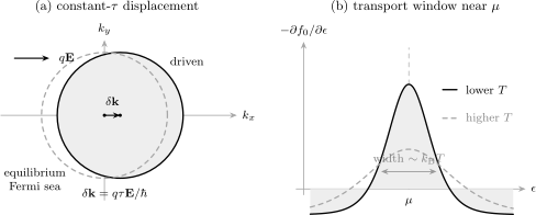
Left: the signed displacement $\delta\mathbf k=q\tau\mathbf E/\hbar$ for the isotropic constant-$\tau$ benchmark. Right: $-\partial f^0/\partial\varepsilon$ restricts degenerate-carrier transport to an energy window of width of order $k_{\mathrm B}T$ around $\mu$; increasing temperature broadens and lowers the normalized window.

Conductivity tensor

The resulting conductivity is

$$\begin{aligned} \sigma_{ij} = q^2 \sum_n \int_{\mathrm{BZ}} \frac{d^dk}{(2\pi)^d} & \tau_{n\mathbf k} v_{n,i}(\mathbf k) v_{n,j}(\mathbf k) \\ &\times \left( - \frac{\partial f^0} {\partial\varepsilon} \right). \end{aligned}$$

All resolved bands contribute. The integrand weights velocity correlation, lifetime, and thermal accessibility, not density of states alone.

For an isotropic parabolic band and constant $\tau$, integration by parts gives

$$\sum_n \int \frac{d^dk}{(2\pi)^d} v_i v_j \left( - \frac{\partial f^0} {\partial\varepsilon} \right) = \frac{n_{\mathrm c}}{m^*} \delta_{ij}.$$

Thus

$$\sigma_{ij} = \frac{ n_{\mathrm c}q^2\tau }{ m^* } \delta_{ij},$$

which recovers Drude Theory as a special reduction.

Transport lifetime

For elastic scattering on an isotropic Fermi surface,

$$\frac{1}{\tau_{\mathrm{tr}}} = \int d\Omega_{\mathbf k'} W_{\mathbf k\to\mathbf k'} \left( 1-\cos\theta \right).$$

The factor $1-\cos\theta$ comes from solving for current relaxation, not from the total escape rate. The quantum or single-particle rate

$$\frac{1}{\tau_q} = \int d\Omega_{\mathbf k'} W_{\mathbf k\to\mathbf k'}$$

counts forward scattering fully. Consequently $\tau_{\mathrm{tr}}$ can greatly exceed $\tau_q$.

Thermal Gradients and Thermoelectric Response

For a weak temperature gradient, the local-equilibrium streaming term adds an energy-dependent drive. In the relaxation-time approximation,

$$\begin{aligned} \phi_{n\mathbf k} = \tau_{n\mathbf k} \mathbf v_{n\mathbf k} \cdot \left[ q\boldsymbol{\mathcal E} - \frac{ \varepsilon_{n\mathbf k}-\mu }{T} \boldsymbol\nabla T \right]. \end{aligned}$$

Particles above and below $\mu$ are driven oppositely by $\boldsymbol\nabla T$. That odd energy weighting is why thermopower is sensitive to particle–hole asymmetry.

Transport distribution

Define the transport distribution tensor

$$\begin{aligned} \Xi_{ij}(\epsilon) := \sum_n \int_{\mathrm{BZ}} \frac{d^dk}{(2\pi)^d} & \tau_{n\mathbf k} v_{n,i}(\mathbf k) v_{n,j}(\mathbf k) \\ &\times \delta \left( \epsilon-\varepsilon_{n\mathbf k} \right). \end{aligned}$$

It combines the density of available states with squared velocity and lifetime. A large density-of-states peak can contribute little to conductivity if the corresponding states are flat or short lived.

Define energy moments

$$\mathcal L_{ij}^{(r)} = \int d\epsilon\, \left( \epsilon-\mu \right)^r \left( - \frac{\partial f^0} {\partial\epsilon} \right) \Xi_{ij}(\epsilon).$$

At zero magnetic field,

$$\mathbf j = q^2 \boldsymbol{\mathcal L}^{(0)} \boldsymbol{\mathcal E} - \frac{q}{T} \boldsymbol{\mathcal L}^{(1)} \boldsymbol\nabla T,$$ $$\mathbf j_Q = q \boldsymbol{\mathcal L}^{(1)} \boldsymbol{\mathcal E} - \frac{1}{T} \boldsymbol{\mathcal L}^{(2)} \boldsymbol\nabla T.$$

The electrical conductivity is

$$\boldsymbol\sigma = q^2 \boldsymbol{\mathcal L}^{(0)}.$$

For a scalar or a common principal axis, the open-circuit Seebeck coefficient is defined by

$$S := \left. \frac{\mathcal E} {\nabla T} \right\rvert_{\mathbf j=0} = \frac{1}{qT} \frac{ \mathcal L^{(1)} }{ \mathcal L^{(0)} }.$$

This agrees with the common voltage convention $S=-\Delta V/\Delta T$ because $\mathcal E=-\boldsymbol\nabla V$ when the chemical contribution is fixed.

The electronic thermal conductivity measured at zero electric current is

$$\boldsymbol\kappa_e = \frac{1}{T} \left[ \boldsymbol{\mathcal L}^{(2)} - \boldsymbol{\mathcal L}^{(1)} \left( \boldsymbol{\mathcal L}^{(0)} \right)^{-1} \boldsymbol{\mathcal L}^{(1)} \right].$$

Using $\boldsymbol{\mathcal L}^{(2)}/T$ alone corresponds to zero electrochemical field, not open circuit. The subtraction accounts for the field that builds up to cancel charge current.

Mott relation

For a degenerate metal with a smooth scalar $\Xi(\epsilon)$,

$$\mathcal L^{(0)} = \Xi(\mu) + O(T^2),$$ $$\mathcal L^{(1)} = \frac{\pi^2}{3} \left( k_{\mathrm B}T \right)^2 \Xi'(\mu) + O(T^4).$$

Therefore

$$S \approx \frac{ \pi^2k_{\mathrm B}^2T }{ 3q } \left. \frac{d\ln\Xi} {d\epsilon} \right\rvert_{\mu}.$$

For electrons, $q=-e$, so a transport distribution increasing with energy gives negative thermopower. The sign is not universally determined by the word electron: multiband compensation, energy-dependent scattering, and nearby singularities can reverse it.

Wiedemann–Franz limit

The same expansion gives

$$\mathcal L^{(2)} = \frac{\pi^2}{3} \left( k_{\mathrm B}T \right)^2 \Xi(\mu) + O(T^4).$$

Hence

$$\frac{\kappa_e}{\sigma T} \longrightarrow L_0, \qquad L_0 = \frac{\pi^2}{3} \left( \frac{k_{\mathrm B}}{e} \right)^2.$$

This limit requires degenerate carriers and sufficiently elastic, smooth transport near $\mu$. Phonon heat conduction, bipolar diffusion, inelastic scattering, hydrodynamic flow, and non-Fermi-liquid dynamics can invalidate a naive comparison.

Metals

At low temperature,

$$- \frac{\partial f^0} {\partial\varepsilon} \longrightarrow \delta \left( \varepsilon-\mu \right).$$

The conductivity becomes a Fermi-surface integral:

$$\begin{aligned} \sigma_{ij} = q^2 \sum_n \int_{\mathrm{FS}_n} \frac{dS}{ (2\pi)^d\hbar } \frac{ \tau_{n\mathbf k} v_{n,i}v_{n,j} }{ |\mathbf v_n| }. \end{aligned}$$

Transport in a metal is therefore organized by the geometry, velocity, and scattering around the Fermi Surface, rather than by all occupied electrons equally.

Typical scattering regimes

• Elastic disorder: produces a residual resistivity to leading order, but anisotropic or resonant defects can make $\tau(\mathbf k,\epsilon)$ strongly structured.
• Acoustic phonons: in a simple three-dimensional metal, the Bloch–Grüneisen result crosses from $\rho_{\mathrm{ph}}\propto T^5$ at low temperature to approximately linear $T$ above the characteristic phonon scale. Dimensionality, screening, Fermi-surface geometry, and phonon spectrum change these powers.
• Electron–electron scattering: a Fermi-liquid quasiparticle rate often scales as $T^2$, but electrical resistivity requires current relaxation through Umklapp, multiband drag, compensation, disorder-assisted processes, or another momentum sink.
• Boundaries: matter when the mean free path approaches a sample dimension; scattering specularity and geometry then enter.

Phonons owns the material lattice modes and electron–phonon kinematics. Lifetime and Spectral Weight distinguishes the transport time from spectral, coherence, and energy-relaxation times.

Matthiessen’s rule,

$$\tau_{\mathrm{tr}}^{-1} \approx \sum_a \tau_a^{-1},$$

is an approximation to the spectrum of a combined collision operator. It is not guaranteed when channels are anisotropic, energy dependent, mutually dressing, or constrained by shared conservation laws.

Semiconductors

In a nondegenerate conduction band,

$$f^0(\epsilon) \approx \exp \left[ - \frac{ \epsilon-\mu }{ k_{\mathrm B}T } \right].$$

Carrier density, mobility, and thermopower can then vary exponentially with chemical potential and sensitively with scattering.

For one isotropic three-dimensional parabolic conduction band,

$$\varepsilon = E_c + \frac{\hbar^2k^2}{2m^*},$$

and a power-law lifetime

$$\tau(\epsilon) \propto \left( \epsilon-E_c \right)^r,$$

the transport distribution scales as

$$\Xi(\epsilon) \propto \left( \epsilon-E_c \right)^{r+3/2}.$$

The nondegenerate thermopower is

$$S_n = \frac{1}{qT} \left[ E_c-\mu + \left( r+\frac{5}{2} \right) k_{\mathrm B}T \right].$$

For electrons $q=-e$, this expression is negative. The constant $5/2$ is specific to a three-dimensional parabolic band and the stated definition of $r$.

Mobility is model dependent

The drift mobility

$$\mu_{\mathrm d} = \frac{\sigma} {n_{\mathrm c}|q|}$$

is an average over the occupied transport distribution. It need not equal $|q|\tau/m^*$ evaluated at a single energy. Valley degeneracy, anisotropic masses, nonparabolicity, ionized-impurity scattering, polar optical phonons, and intervalley transitions can all change the average.

Electrons and holes together

For independent electron and hole channels,

$$\sigma = \sigma_n+\sigma_p,$$

and

$$S = \frac{ \sigma_nS_n+\sigma_pS_p }{ \sigma_n+\sigma_p }.$$

Opposite thermopower signs can cancel even when both carrier populations are large. Bipolar diffusion also adds heat conduction, so an intrinsic semiconductor can violate a one-carrier Wiedemann–Franz estimate without exotic physics.

Magnetic Field and Chambers Formula

At nonzero magnetic field, the Lorentz term moves a quasiparticle along a constant-energy orbit:

$$\hbar\dot{\mathbf k} = q \mathbf v_n(\mathbf k) \times \mathbf B.$$

For one band with constant $\tau$, the formal steady solution leads to Chambers’ formula:

$$\begin{aligned} \sigma_{ij}(\mathbf B) = q^2 \int_{\mathrm{BZ}} \frac{d^dk}{(2\pi)^d} & \left( - \frac{\partial f^0} {\partial\varepsilon} \right) v_i\!\left[ \mathbf k(0) \right] \\ &\times \int_{-\infty}^{0} dt\, e^{t/\tau} v_j\!\left[ \mathbf k(t) \right]. \end{aligned}$$

The current at the present state remembers the velocity history over approximately one relaxation time. At $\mathbf B=0$, $\mathbf k(t)$ is constant and the inner integral becomes $\tau v_j$.

This expression exposes why magnetotransport depends on whole Fermi-surface orbits, open trajectories, and anisotropic lifetimes. The elementary isotropic Hall tensor is derived in Drude Theory; a full Hall analysis must also track tensor inversion, multiband response, Berry curvature, and magnetization-current conventions.

Conservation, Entropy, and Reciprocity

Define the weighted inner product

$$\langle a,b\rangle = \sum_n \int_{\mathrm{BZ}} \frac{d^dk}{(2\pi)^d} \left( - \frac{\partial f^0} {\partial\varepsilon} \right) a_{n\mathbf k} b_{n\mathbf k}.$$

For a detailed-balance collision operator,

$$\langle\phi,\mathcal C\phi\rangle \ge 0.$$

Up to convention-dependent normalization, this quadratic form is $T$ times the collision-generated entropy-production rate. Equality identifies a collision invariant.

This structure supports variational solutions: trial functions give controlled approximations to the current-carrying deformation when the null modes are handled correctly. It also makes a negative longitudinal conductivity from a passive, equilibrium, linearized calculation a diagnostic of a sign, discretization, or collision-kernel error.

Microscopic reversibility implies Onsager–Casimir relations. For example,

$$\sigma_{ij}(\mathbf B) = \sigma_{ji}(-\mathbf B).$$

Thermoelectric cross coefficients obey corresponding relations after current definitions and time-reversal parities are matched. A numerical solver should recover these symmetries within convergence error.

When the Semiclassical Theory Is Controlled

Several conditions are logically separate:

Requirement	Practical diagnostic	Failure sign
resolved quasiparticle	spectral width small relative to the local dispersion or band separation	broad incoherent continuum
slow spatial variation	mean free path and packet size small relative to device or gradient scale	nonlocal or ballistic response
weak drive	field work over a mean free path small relative to the equilibrium energy window	carrier heating or nonlinear distribution
Markovian collisions	collision duration and memory short relative to evolution time	frequency-dependent memory kernel
semiclassical magnetic motion	Landau quantization and magnetic breakdown negligible	quantum oscillations or discrete levels
continuum state sampling	many states in the relevant thermal and disorder window	finite-size level sensitivity
negligible coherent interference	phase coherence not controlling return probability	weak or strong localization

Useful inequalities include

$$\ell_{\mathrm{tr}} \ll L_{\mathrm{drive}},$$ $$|q\mathcal E| \ell_{\mathrm{tr}} \ll E_{\mathrm{window}},$$

and, when a smooth magnetic orbit is assumed,

$$\hbar|\omega_c| \ll \max \left( k_{\mathrm B}T, \Gamma_E \right)$$

if Landau quantization is to remain unresolved. The relevant energy window depends on whether the carriers are degenerate, activated, multiband, or near a band edge.

Important breakdowns

• Hydrodynamic regime: fast momentum-conserving collisions establish local equilibrium. A single-state RTA destroys the conserved modes that hydrodynamics requires.
• Ballistic or mesoscopic regime: leads, contacts, and transmission eigenvalues replace a local bulk resistivity. See Conductance Quantization for the channel ledger and Mesoscopic Transport for the open-system viewpoint.
• Localization: coherent multiple scattering changes diffusion and cannot be reconstructed from independent transition probabilities.
• Strongly incoherent matter: no sharply defined band quasiparticle distribution may exist.
• Interband coherence: nearly degenerate bands can require a density-matrix or quantum kinetic equation rather than scalar occupations.
• Ultrafast driving: memory, coherent polarization, and time-dependent self-energies can matter before a Markov collision integral is established.

Fermi-Liquid Theory Preview develops the interacting quasiparticle kinetic equation. Hydrodynamics as an Effective Theory owns the long-wavelength theory after nonconserved distortions have relaxed.

Solving Beyond a Constant Relaxation Time

A material calculation can proceed at several levels:

1. Constant relaxation time: isolates band-structure weighting but does not predict absolute conductivity.
2. State-dependent diagonal lifetime: includes energy, band, and momentum dependence while discarding scattering in.
3. Momentum-relaxation approximation: inserts angular current-loss factors in a restricted geometry.
4. Iterative linearized Boltzmann equation: solves the coupled scattering-in problem.
5. Variational solution: optimizes a trial space using positivity of the collision operator.
6. Quantum kinetic or Kubo treatment: retains coherence, off-shell structure, or vertex information beyond a classical distribution.

Reproducible workflow

A trustworthy numerical report should state:

• the electronic bands, quasiparticle corrections, and interpolation method;
• the velocity convention and treatment of degeneracies;
• the scattering mechanisms and matrix elements;
• energy and momentum delta-function regularization;
• phonon occupations and absorption/emission balance;
• whether the solution is constant-$\tau$, diagonal, momentum-relaxation, iterative, or variational;
• Brillouin-zone meshes for electrons and phonons;
• chemical potential, carrier density, temperature, dimensional normalization, and sample volume convention;
• convergence of conductivity, mobility, and thermopower separately;
• conservation, detailed-balance, positivity, and reciprocity checks.

Thermopower can appear converged while conductivity is not, because $S$ is a ratio of moments and a constant $\tau$ cancels. That cancellation does not validate the assumed scattering physics.

Common Mistakes

• Calling $f_n(\mathbf k)$ a wavefunction or probability amplitude.
• Multiplying by spin or valley degeneracy after those states were already summed explicitly.
• Using the total escape lifetime in place of a transport lifetime.
• Omitting Pauli blocking or inverse phonon processes.
• Applying a diagonal RTA to a conserved density mode.
• Inferring resistivity from electron–electron collision frequency without checking momentum and current overlap.
• Treating density of states alone as a conductivity measure.
• Using $\mathcal L^{(2)}/T$ as the open-circuit thermal conductivity.
• Dropping the signed charge in thermopower and Hall formulas.
• Reporting $\sigma/\tau$ from a constant-$\tau$ code as an absolute conductivity.
• Combining rates by Matthiessen’s rule without testing the full angular or energy dependence.
• Using semiclassical orbits after Landau quantization is resolved.
• Applying bulk Boltzmann theory when contacts or phase coherence control the measured conductance.
• Comparing a calculated transport time directly with an ARPES or quantum-oscillation lifetime.

Exercises

1. Recover the Drude conductivity

For an isotropic parabolic band with constant $\tau$, use integration by parts in $\mathbf k$ to prove

$$\sigma_{ij} = \frac{n_{\mathrm c}q^2\tau}{m^*} \delta_{ij}.$$

Solution

Since

$$\frac{\partial f^0} {\partial k_i} = \hbar v_i \frac{\partial f^0} {\partial\varepsilon},$$

we have

$$\begin{aligned} \int \frac{d^dk}{(2\pi)^d} v_iv_j \left( - \frac{\partial f^0} {\partial\varepsilon} \right) &= - \frac{1}{\hbar} \int \frac{d^dk}{(2\pi)^d} v_j \frac{\partial f^0} {\partial k_i} \\ &= \frac{1}{\hbar} \int \frac{d^dk}{(2\pi)^d} f^0 \frac{\partial v_j} {\partial k_i}. \end{aligned}$$

For $\varepsilon=\hbar^2k^2/(2m^*)$,

$$\frac{\partial v_j} {\partial k_i} = \frac{\hbar}{m^*} \delta_{ij}.$$

The remaining integral is $n_{\mathrm c}$, so inserting the result into the conductivity tensor gives the stated Drude form.

2. Audit number conservation in the RTA

Let

$$\delta f_a = C \left( - \frac{\partial f_a^0} {\partial\varepsilon_a} \right)$$

represent a small uniform chemical-potential shift. Does $\mathcal I_a=-\delta f_a/\tau$ conserve particle number for constant $\tau$?

Solution

The integrated collision term is

$$\sum_a \mathcal I_a = - \frac{C}{\tau} \sum_a \left( - \frac{\partial f_a^0} {\partial\varepsilon_a} \right).$$

The sum is positive for a compressible system, so the result is nonzero. The diagonal RTA incorrectly relaxes a uniform density shift into or out of existence.

A conserving model must relax toward a local equilibrium $f_{\mathrm{le}}$ with a shifted chemical potential chosen so that

$$\sum_a \left( f_a-f_{\mathrm{le},a} \right) = 0.$$

3. Angular scattering

In two dimensions, take an elastic angular kernel

$$W(\theta) = W_0 \left( 1+a\cos\theta \right), \qquad |a|\le1.$$

Find $\tau_q^{-1}$ and $\tau_{\mathrm{tr}}^{-1}$ up to the common state-density factor.

Solution

The quantum rate is

$$\begin{aligned} \tau_q^{-1} &= \int_0^{2\pi} d\theta\, W(\theta) \\ &= 2\pi W_0. \end{aligned}$$

The transport rate is

$$\begin{aligned} \tau_{\mathrm{tr}}^{-1} &= \int_0^{2\pi} d\theta\, W(\theta) \left( 1-\cos\theta \right) \\ &= \pi W_0 \left( 2-a \right). \end{aligned}$$

Thus

$$\frac{ \tau_{\mathrm{tr}}^{-1} }{ \tau_q^{-1} } = 1-\frac{a}{2}.$$

Forward-favoring scattering has $a>0$ and relaxes current less efficiently than it broadens a single-particle state.

4. Mott and Wiedemann–Franz limits

Assume a smooth scalar transport distribution. Use

$$\mathcal L^{(0)} \approx \Xi(\mu),$$ $$\mathcal L^{(1)} \approx \frac{\pi^2}{3} \left( k_{\mathrm B}T \right)^2 \Xi'(\mu),$$ $$\mathcal L^{(2)} \approx \frac{\pi^2}{3} \left( k_{\mathrm B}T \right)^2 \Xi(\mu)$$

to obtain $S$ and $\kappa_e/(\sigma T)$ to leading order.

Solution

The thermopower is

$$\begin{aligned} S &= \frac{1}{qT} \frac{ \mathcal L^{(1)} }{ \mathcal L^{(0)} } \\ &\approx \frac{ \pi^2k_{\mathrm B}^2T }{ 3q } \frac{ \Xi'(\mu) }{ \Xi(\mu) }. \end{aligned}$$

The subtraction in $\kappa_e$ is of order $T^3$, while the leading $\mathcal L^{(2)}/T$ term is order $T$. Therefore

$$\kappa_e \approx \frac{\pi^2}{3} k_{\mathrm B}^2T \Xi(\mu).$$

Since $\sigma=q^2\Xi(\mu)$,

$$\frac{\kappa_e}{\sigma T} \approx \frac{\pi^2}{3} \frac{k_{\mathrm B}^2}{q^2} = \frac{\pi^2}{3} \left( \frac{k_{\mathrm B}}{e} \right)^2.$$

5. Nondegenerate semiconductor thermopower

For a three-dimensional parabolic conduction band with $\tau\propto(\epsilon-E_c)^r$, show that

$$\frac{ \mathcal L^{(1)} }{ \mathcal L^{(0)} } = E_c-\mu + \left( r+\frac{5}{2} \right) k_{\mathrm B}T.$$

Solution

The transport distribution is

$$\Xi(\epsilon) \propto x^{r+3/2}, \qquad x=\epsilon-E_c.$$

In the nondegenerate limit, the common weight is proportional to $e^{-x/(k_{\mathrm B}T)}$. The weighted mean of $x$ is

$$\langle x\rangle = \frac{ \int_0^\infty dx\, x^{r+5/2} e^{-x/(k_{\mathrm B}T)} }{ \int_0^\infty dx\, x^{r+3/2} e^{-x/(k_{\mathrm B}T)} } = \left( r+\frac{5}{2} \right) k_{\mathrm B}T,$$

using $\Gamma(z+1)=z\Gamma(z)$. Since $\epsilon-\mu=E_c-\mu+x$, the result follows. Dividing by $qT$ gives the Seebeck coefficient.

6. Two-carrier thermopower

An electron channel has $\sigma_n=3\sigma_0$ and $S_n=-120\,\mu\mathrm{V\,K^{-1}}$. A hole channel has $\sigma_p=\sigma_0$ and $S_p=240\,\mu\mathrm{V\,K^{-1}}$. Find the measured open-circuit thermopower.

Solution

The conductivity-weighted result is

$$\begin{aligned} S &= \frac{ 3\sigma_0 \left( -120 \right) + \sigma_0 \left( 240 \right) }{ 4\sigma_0 } \, \mu\mathrm{V\,K^{-1}} \\ &= -30\, \mu\mathrm{V\,K^{-1}}. \end{aligned}$$

The negative sign does not mean holes are absent. Their positive contribution is outweighed by the more conductive electron channel.

7. Chambers formula at zero field

Show that Chambers’ formula reduces to the relaxation-time conductivity when $\mathbf B=0$.

Solution

At zero magnetic field,

$$\mathbf k(t) = \mathbf k(0),$$

so

$$\begin{aligned} \int_{-\infty}^{0} dt\, e^{t/\tau} v_j \left[ \mathbf k(t) \right] &= v_j(\mathbf k) \int_{-\infty}^{0} dt\, e^{t/\tau} \\ &= \tau v_j(\mathbf k). \end{aligned}$$

Substitution gives

$$\sigma_{ij} = q^2 \int \frac{d^dk}{(2\pi)^d} \tau v_iv_j \left( - \frac{\partial f^0} {\partial\varepsilon} \right),$$

which is the zero-field relaxation-time result.

Connections

• Transport Measurements supplies the four-terminal, geometry, sweep, and uncertainty contract required before a measured resistance is compared with a kinetic transport coefficient.
• Conductance Quantization develops the ballistic channel description that replaces the local collision equation in a short constriction.
• Drude Theory is recovered for one isotropic parabolic band with constant transport time.
• Disorder in Quantum Matter connects impurity correlators to differential scattering, quantum and transport lifetimes, and the regime parameter $k_{\mathrm F}\ell$.
• Superconducting Proximity Effect uses normal-state mean free paths and diffusion constants diagnosed here to choose clean or dirty quasiclassical propagation; anomalous Green functions and superconducting self-consistency remain outside Boltzmann kinetics.
• Hall Effect applies finite-field kinetic response to carrier sign, multiband transport, anomalous Hall mechanisms, and measured tensors.
• Fermi Surface supplies the low-temperature geometry, velocities, pockets, and orbit structure.
• Density of States develops state-counting measures; Boltzmann transport adds velocity and lifetime weighting.
• Effective Mass distinguishes curvature, conductivity, density-of-states, cyclotron, and optical masses.
• Phonons supplies lattice modes and electron–phonon kinematics.
• Kondo Effect shows how scale-dependent spin-flip scattering produces a resistivity minimum and escapes a constant relaxation-time description.
• Spintronics adds spin-resolved diffusion, injection boundary conditions, nonlocal detection, and interfacial torque to the charge-transport baseline.
• Kubo Formula gives the exact linear-response framework and the diagrammatic meaning of transport vertex corrections.
• Strange Metals compares anomalous low-temperature linear resistivity with the phonon, hot–cold, and multiband baselines developed here.
• Transport Coefficients Preview treats diffusion, hydrodynamics, Green–Kubo relations, and orders of limits.
• Condensed Matter Roadmap places kinetic theory between band structure and more general response and mesoscopic methods.

References

• L. Boltzmann, “Weitere Studien über das Wärmegleichgewicht unter Gasmolekülen,” Sitzungsberichte der Kaiserlichen Akademie der Wissenschaften, Mathematisch-Naturwissenschaftliche Classe 66, 275–370 (1872).
• N. W. Ashcroft and N. D. Mermin, Solid State Physics, Holt, Rinehart and Winston, 1976.
• J. M. Ziman, Electrons and Phonons: The Theory of Transport Phenomena in Solids, Oxford University Press, 1960; Oxford Classic Texts reissue, 2001, doi:10.1093/acprof:oso/9780198507796.001.0001.
• R. G. Chambers, “The Kinetic Formulation of Conduction Problems,” Proceedings of the Physical Society. Section A 65, 458–459 (1952), doi:10.1088/0370-1298/65/6/114.
• L. Onsager, “Reciprocal Relations in Irreversible Processes. I,” Physical Review 37, 405–426 (1931), doi:10.1103/PhysRev.37.405.
• L. Onsager, “Reciprocal Relations in Irreversible Processes. II,” Physical Review 38, 2265–2279 (1931), doi:10.1103/PhysRev.38.2265.
• M. Cutler and N. F. Mott, “Observation of Anderson Localization in an Electron Gas,” Physical Review 181, 1336–1340 (1969), doi:10.1103/PhysRev.181.1336.
• M. Jonson and G. D. Mahan, “Mott’s Formula for the Thermopower and the Wiedemann–Franz Law,” Physical Review B 21, 4223–4229 (1980), doi:10.1103/PhysRevB.21.4223.
• S. Poncé, W. Li, S. Reichardt, and F. Giustino, “First-Principles Calculations of Charge Carrier Mobility and Conductivity in Bulk Semiconductors and Two-Dimensional Materials,” Reports on Progress in Physics 83, 036501 (2020), doi:10.1088/1361-6633/ab6a43.
• M. Battiato, V. Zlatić, and K. Held, “Boltzmann Approach to High-Order Transport: The Nonlinear and Nonlocal Responses,” Physical Review B 95, 235137 (2017), doi:10.1103/PhysRevB.95.235137.