Semiclassical Dynamics of Bloch Electrons

Semiclassical Bloch dynamics represents a quantum state localized in both real space and crystal momentum by a center $(\mathbf r_c,\mathbf k_c)$ that moves through one isolated band. In the ordinary, nongeometric approximation, a carrier of signed charge $q$ obeys

$$\dot{\mathbf r}_c = \frac{1}{\hbar} \nabla_{\mathbf k} \varepsilon_n(\mathbf k_c), \qquad \hbar\dot{\mathbf k}_c = q \left( \mathbf E + \dot{\mathbf r}_c\times\mathbf B \right).$$

For an electron, $q=-e$ with $e>0$; for a hole described relative to a filled band, $q=+e$. The first equation is a property of the band dispersion. The second is the Lorentz-force law for crystal momentum. Neither equation supplies a collision time, a conductivity, a Landau spectrum, or a guarantee that one band remains isolated.

Electromagnetic equations on this page use SI units. In Gaussian units the magnetic Lorentz term carries the corresponding factor of $1/c$.

Here $\mathbf k_c$ is a wave-vector coordinate on the Brillouin torus, not the electron’s mechanical momentum divided by $\hbar$. This page owns the construction and controlled use of the one-band packet, including uniform electric and magnetic fields and explicit failure tests. Effective Mass owns the taxonomy of mass parameters; Fermi Surface owns constant-energy sheet and orbit geometry; Boltzmann Transport owns distributions and collisions; and the canonical Landau Levels page owns resolved orbital quantization.

Required background. Band Theory Overview supplies Bloch states, band energies, Brillouin-zone periodicity, and the distinction among model, Kohn–Sham, and coherent quasiparticle bands.

Helpful background. Wave Packets and Classical Trajectories supplies generic localization, spreading, and trajectory criteria, while Effective Mass supplies the local band Hessian. General Berry Curvature is needed only for the geometric branch below.

An Isolated-Band Wave Packet

Let a periodic Hamiltonian have normalized cell-periodic eigenvectors

$$H(\mathbf k) |u_{n\mathbf k}\rangle = \varepsilon_n(\mathbf k) |u_{n\mathbf k}\rangle,$$

and Bloch states $|\psi_{n\mathbf k}\rangle$. A packet made from one band is

$$|W_n\rangle = \int_{\mathrm{BZ}}[d\mathbf k]\, a(\mathbf k,t) |\psi_{n\mathbf k}\rangle, \qquad \int_{\mathrm{BZ}}[d\mathbf k]\, |a(\mathbf k,t)|^2 = 1,$$

where $[d\mathbf k]$ and the normalization of the Bloch states are chosen consistently. The envelope is concentrated in a contractible patch around $\mathbf k_c$. Within that patch one may define

$$\mathbf k_c = \int_{\mathrm{BZ}}[d\mathbf k]\, |a(\mathbf k,t)|^2\mathbf k, \qquad \mathbf r_c = \langle W_n|\mathbf r|W_n\rangle.$$

The first formula is not a global average of angular coordinates across an arbitrary Brillouin-zone cut; it is meaningful because the packet is narrow in a local chart. If $a=|a|e^{-i\gamma}$, the narrow-packet center has the local form

$$\mathbf r_c \simeq \nabla_{\mathbf k}\gamma(\mathbf k_c) + \boldsymbol{\mathcal A}_n(\mathbf k_c), \qquad \boldsymbol{\mathcal A}_n = i \langle u_{n\mathbf k}| \nabla_{\mathbf k}u_{n\mathbf k}\rangle.$$

The two terms change oppositely under a Bloch-state gauge transformation, so their sum is gauge invariant. This is a local construction: a packet can be assembled patchwise even when no globally smooth eigenvector exists over the full Brillouin zone.

Let $a_{\mathrm{lat}}$ denote a representative lattice spacing, $L_{\mathrm{pert}}$ the shortest spatial scale on which the external perturbation changes appreciably, and $\Delta r_i$, $\Delta k_i$ the rms standard deviations along a chosen pair of conjugate directions. A controlled local packet requires a window such as

$$a_{\mathrm{lat}} \ll \Delta r \ll L_{\mathrm{pert}}, \qquad L_{\mathrm{pert}}^{-1} \ll \Delta k \ll a_{\mathrm{lat}}^{-1}, \qquad \Delta r_i\Delta k_i \gtrsim \frac12.$$

The packet spans many cells, so microscopic lattice oscillations are averaged into a band description, but it remains small enough to sample the perturbation locally. It must also remain in one spectrally isolated band over its significant momentum region and over the trajectory it will explore. A narrow packet centered far from a degeneracy can be valid even if the band touches another band elsewhere in the Brillouin zone; a trajectory through that touching cannot.

A Gaussian envelope has nonzero mathematical tails throughout the Brillouin zone, so literal support is too strong for a practical isolation test. Fix a small discarded-weight tolerance $\delta_a$ and declare a significant-weight region $\mathcal K_a(t)$ such that

$$\int_{\mathrm{BZ}\setminus\mathcal K_a(t)} [d\mathbf k]\, |a(\mathbf k,t)|^2 < \delta_a.$$

Whenever this page refers to the packet’s retained momentum region, it means the declared $\mathcal K_a(t)$ together with the reported tolerance, not the literal support of an infinite-tailed model envelope.

Group Velocity in a Bloch Band

Without external perturbations, each momentum component accumulates the phase $\exp[-i\varepsilon_n(\mathbf k)t/\hbar]$. Expanding that phase around $\mathbf k_c$ translates the packet envelope at

$$\mathbf v_n(\mathbf k_c) = \frac{1}{\hbar} \nabla_{\mathbf k} \varepsilon_n(\mathbf k_c).$$

More precisely, before replacing the packet by its center,

$$\dot{\mathbf r}_c = \int_{\mathrm{BZ}}[d\mathbf k]\, |a(\mathbf k,t)|^2 \mathbf v_n(\mathbf k).$$

The center formula follows when $\mathbf v_n$ varies little across the support. Packet spreading and distortion depend on higher derivatives and are not encoded by the center alone.

For a local Schrödinger Hamiltonian,

$$H(\mathbf k) = \frac{(\mathbf p+\hbar\mathbf k)^2}{2m} +V(\mathbf r),$$

the Hellmann–Feynman theorem gives

$$\frac{1}{\hbar} \frac{\partial\varepsilon_n}{\partial k_i} = \frac{1}{\hbar} \left\langle u_{n\mathbf k}\middle| \frac{\partial H(\mathbf k)}{\partial k_i} \middle|u_{n\mathbf k}\right\rangle = \left\langle \frac{p_i+\hbar k_i}{m} \right\rangle.$$

Thus the gradient of the band energy is the cell-averaged physical velocity for that Bloch state. It need not be parallel to $\mathbf k$, and it is periodic under $\mathbf k\mapsto\mathbf k+\mathbf G$. A flat band has vanishing ordinary group velocity even though its Bloch eigenvectors may carry nontrivial geometry.

Crystal Momentum Under Force

For an electric field alone, the acceleration theorem is

$$\hbar\dot{\mathbf k}_c = q\mathbf E.$$

A uniform field therefore translates the packet through reciprocal space at a rate whose direction already contains the carrier-sign convention. An electron moves opposite $\mathbf E$ in $\mathbf k$ space. In a reduced-zone description, crossing a chosen zone face merely changes the representative by a reciprocal vector; it is not automatically an interband transition.

In slowly varying electromagnetic fields, the ordinary coupled equations are

$$\begin{aligned} \dot{\mathbf r}_c &= \frac{1}{\hbar} \nabla_{\mathbf k} \varepsilon_n(\mathbf k_c), \\ \hbar\dot{\mathbf k}_c &= q \left[ \mathbf E(\mathbf r_c,t) + \dot{\mathbf r}_c\times \mathbf B(\mathbf r_c,t) \right]. \end{aligned}$$

An additional smooth scalar energy $U(\mathbf r)$ contributes $-\nabla_{\mathbf r}U$ to the second equation. If $U=q\phi$ already represents the electrostatic energy, its force is $q\mathbf E$ and must not be counted twice.

The energy ledger is an immediate consistency check:

$$\begin{aligned} \frac{d\varepsilon_n}{dt} &= \nabla_{\mathbf k}\varepsilon_n \cdot\dot{\mathbf k}_c \\ &= q\, \dot{\mathbf r}_c\cdot\mathbf E. \end{aligned}$$

The magnetic part vanishes because $\dot{\mathbf r}_c\cdot(\dot{\mathbf r}_c\times\mathbf B)=0$. A magnetic field redirects an ordinary band trajectory but does no work; an electric field changes the band energy at the rate charge times electric power per unit charge.

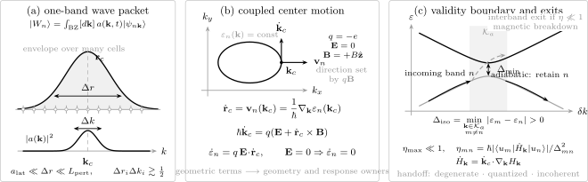
A Bloch wave packet must span many unit cells while remaining small compared with the perturbation scale. Within an isolated band, its center follows the ordinary group-velocity and Lorentz-force equations, where $q$ is the signed carrier charge; a magnetic field alone moves the packet along a constant-energy contour. The one-band description additionally requires a nonzero separation over the declared significant-weight region and small nonadiabatic coupling. Degeneracies, Landau–Zener transitions, magnetic breakdown, resolved Landau quantization, or loss of a coherent quasiparticle require the corresponding multiband, quantized, or spectral treatment.

Uniform Electric Fields and Bloch Oscillations

Set $\mathbf B=0$ and take $\mathbf E$ constant. Then

$$\mathbf k_c(t) = \mathbf k_c(0) + \frac{q\mathbf E}{\hbar}t,$$

with reciprocal-lattice equivalence understood. Because $\varepsilon_n(\mathbf k)$ is periodic on the Brillouin torus, the velocity repeats whenever the trajectory advances by a reciprocal vector. In one dimension, a perfectly coherent isolated band therefore produces Bloch oscillations rather than indefinite acceleration. No physical reflection at a zone boundary is required.

In more than one dimension, a finite recurrence time exists only when the field direction is commensurate with the reciprocal lattice: for some nonzero reciprocal vector $\mathbf G$,

$$\frac{q\mathbf E T}{\hbar} = \mathbf G.$$

An incommensurate direction generally gives quasiperiodic velocity, and even a closed reciprocal-space path can carry an ordinary transverse drift. The one-dimensional example below has an unambiguous period and zero displacement over a complete cycle.

Worked one-dimensional tight-binding band

For lattice spacing $a$ and hopping energy $J>0$, consider

$$\varepsilon(k) = -2J\cos(ka).$$

The group velocity and accelerated wave vector are

$$v(k) = \frac{2Ja}{\hbar}\sin(ka), \qquad k(t) = k_0+ \frac{qE}{\hbar}t.$$

One reciprocal period $2\pi/a$ is traversed in the Bloch period

$$T_B = \frac{2\pi\hbar}{|qE|a} = \frac{h}{|qE|a}.$$

Integrating the velocity gives

$$\begin{aligned} x(t)-x(0) &= \frac{\varepsilon[k(t)]-\varepsilon(k_0)}{qE} \\ &= \frac{2J}{qE} \left[ \cos(k_0a)-\cos(k(t)a) \right]. \end{aligned}$$

The peak-to-peak excursion is $4J/|qE|$, and the time average of $v$ over one full period is zero. This is a coherent single-band result, not a generic prediction of zero current in a real crystal. Scattering interrupts the cycle, interband transfer leaks amplitude into other bands, and geometric terms can add transverse motion. Those effects require their own declared regimes.

Uniform Magnetic Fields and Band Orbits

Set $\mathbf E=0$ and take $\mathbf B$ constant. The equations imply two invariants:

$$\frac{d\varepsilon_n}{dt} = 0, \qquad \frac{d}{dt} \left( \widetilde{\mathbf k}_c\cdot\mathbf B \right) = 0.$$

Here $\widetilde{\mathbf k}_c(t)$ is a continuous lift of the trajectory to repeated-zone reciprocal space. The dot product is not a globally single-valued coordinate on the Brillouin torus because adding $\mathbf G$ can change it. The lifted trajectory is the intersection of a periodically continued constant-energy surface with a plane perpendicular to $\mathbf B$; the physical torus path is its projection modulo reciprocal vectors. The signed charge fixes its orientation. Closed and open projected paths have different dynamical consequences, but their classification and extremal areas belong to Fermi Surface.

For $\mathbf B=B\hat{\mathbf z}$, the transverse real- and reciprocal-space displacements satisfy locally

$$\mathbf r_{c\perp}(t)-\mathbf r_{c\perp}(0) = \frac{\hbar}{qB} \hat{\mathbf z}\times \left[ \widetilde{\mathbf k}_{c\perp}(t)- \widetilde{\mathbf k}_{c\perp}(0) \right].$$

Weak field has more than one meaning. The magnetic length

$$\ell_B = \sqrt{ \frac{\hbar}{|q|\,|\mathbf B|} }$$

should be large compared with microscopic lattice scales for a local band trajectory. Equivalently, for a representative cell cross-section $A_c$, the flux test is

$$\frac{|q|\,|\mathbf B|A_c}{h} \ll 1.$$

The field-driven orbit must also avoid appreciable transfer to nearby bands. Separately, discrete Landau levels become spectrally resolved when a representative spacing $\hbar\omega_c$ is comparable to or larger than both thermal broadening $k_{\mathrm B}T$ and a disorder linewidth $\Gamma$. At that point a continuous phase-space trajectory is no longer a sufficient description of the spectrum. Landau Levels in Solids owns the controlled promotion from a local material band Hamiltonian to that resolved ladder. Quantum Oscillations owns orbit-to-data inference, while Landau Levels and Magnetic Translations retain the canonical spectrum and field-modified translation algebra.

The Effective-Mass Handoff

Differentiate the group velocity along the trajectory. With the local inverse curvature tensor

$$\left( \mathsf M_n^{-1} \right)_{ij} = \frac{1}{\hbar^2} \frac{\partial^2\varepsilon_n} {\partial k_i\partial k_j},$$

the ordinary acceleration is

$$\dot v_i = \sum_j \left( \mathsf M_n^{-1} \right)_{ij} F_j, \qquad \mathbf F = \hbar\dot{\mathbf k}_c.$$

This equation is local: both the Hessian and the force are evaluated along the path. Force and acceleration need not be parallel in an anisotropic band, and a constant force need not produce constant acceleration in a nonparabolic band. Negative electron-band curvature is not by itself a positive carrier charge. Effective Mass owns curvature, conductivity, density-of-states, cyclotron, optical, and quasiparticle masses; Holes owns the positive-charge reorganization near a full band.

Berry Curvature and Orbital-Moment Handoff

The ordinary equations depend only on $\varepsilon_n(\mathbf k)$. A wave packet also samples how $|u_{n\mathbf k}\rangle$ changes across momentum space. With the connection convention introduced above, define

$$\boldsymbol\Omega_n = \nabla_{\mathbf k} \times \boldsymbol{\mathcal A}_n.$$

For an isolated nondegenerate band in spatially uniform fields, the leading geometric form is

$$\dot{\mathbf r}_c = \frac{1}{\hbar} \nabla_{\mathbf k} \widetilde{\varepsilon}_n - \dot{\mathbf k}_c\times \boldsymbol\Omega_n,$$

where $\boldsymbol\Omega_n$ is the Berry curvature and

$$\widetilde{\varepsilon}_n = \varepsilon_n - \mathbf m_n\cdot\mathbf B$$

includes the band orbital magnetic moment. The force equation remains coupled to $\dot{\mathbf r}_c$, so the system must be solved consistently. In an inhomogeneous field, $-\nabla_{\mathbf r_c}\widetilde{\varepsilon}_n$ must also enter $\hbar\dot{\mathbf k}_c$; the uniform-field preview does not include that force.

The same first-order expansion changes the phase-space factor to

$$D_n = 1 - \frac{q}{\hbar} \mathbf B\cdot\boldsymbol\Omega_n.$$

This preview is not a license to append only an anomalous-velocity term to an otherwise ordinary calculation. At the same order, the orbital moment, field-corrected energy, phase-space measure, occupation, magnetization currents, and observable-current definition may matter. General Berry Curvature owns the gauge geometry, and Hall Effect owns the distinction among intrinsic, scattering-dependent, and measured transverse response. Local nonzero curvature is not by itself a Chern number or a Hall coefficient.

When One Band Is Not Enough

An isolated band must remain separated over the declared significant-weight region, not merely at its center. A useful instantaneous gap is

$$\Delta_{\mathrm{iso}}(t) = \min_{\substack{ \mathbf k\in\mathcal K_a(t)\\ m\ne n }} \left| \varepsilon_m(\mathbf k) - \varepsilon_n(\mathbf k) \right|.$$

One needs $\Delta_{\mathrm{iso}}>0$ along the full trajectory. Gap size alone is not enough; the rate at which the basis changes also matters. For $m\ne n$, define the local adiabatic diagnostic

$$\eta_{mn}(\mathbf k,t) = \frac{ \hbar \left| \dot{\mathbf k}_c\cdot \langle u_{m\mathbf k}| \nabla_{\mathbf k}H(\mathbf k) |u_{n\mathbf k}\rangle \right| }{ |\varepsilon_m(\mathbf k)-\varepsilon_n(\mathbf k)|^2 }, \qquad \eta_{\max}(t) = \max_{\substack{ \mathbf k\in\mathcal K_a(t)\\ m\ne n }} \eta_{mn}(\mathbf k,t).$$

Single-band following requires $\eta_{\max}\ll1$ together with a discarded tail small enough that it does not change the requested observable. This instantaneous ratio is a useful local warning, not by itself a rigorous long-time error bound; smoothness, accumulated duration, and packet spreading must also be controlled. At an exact degeneracy, an individual-band eigenvector is not a unique smooth object and this ratio is singular; the retained object must be a multiband subspace.

Near an isolated avoided crossing, write the local projected Hamiltonian in a diabatic basis as

$$H_{\mathrm{loc}}(\mathbf k) = \frac{\delta(\mathbf k)}{2}\sigma_z + \Delta\sigma_x.$$

The minimum adiabatic gap is $2|\Delta|$. The band-dynamics problem supplies the diabatic sweep rate

$$\alpha = \left. \frac{d\delta}{dt} \right|_{\mathbf k_c} = \dot{\mathbf k}_c\cdot \nabla_{\mathbf k}\delta, \qquad \mathbf B=0 \ \Longrightarrow\ \alpha = \frac{q}{\hbar} \mathbf E\cdot \nabla_{\mathbf k}\delta.$$

The Landau–Zener Transition page takes $|\alpha|$ and $|\Delta|$ as inputs and owns the asymptotic transition probability, basis convention, finite-window audit, and extensions. In a magnetic field, two nearby semiclassical orbits can undergo analogous field-driven transfer across a small band gap. This magnetic breakdown changes the orbit network and cannot be repaired by continuing a single-band path through the junction. Multiple junctions can also interfere coherently.

The principal one-band failure modes are distinct:

Failure	Lost assumption	Required change
exact or symmetry-enforced degeneracy	unique isolated eigenline	propagate the degenerate subspace with a multiband Hamiltonian
electric-field interband transfer	adiabatic following through an avoided crossing	use Landau–Zener or a full time-dependent multiband calculation
magnetic breakdown	orbit remains on one sheet	use a coupled orbit network with junction amplitudes
resolved orbital quantization	continuous phase-space spectrum	use Landau-level or magnetic-translation methods
packet splitting across branches	one localized center represents the state	propagate multiple packets or the full state

Strong field is therefore not one universal threshold. Interband transfer, magnetic breakdown, and resolved intraband quantization compare the field with different gaps, velocities, broadenings, and length scales.

Disorder, Collisions, and Spectral Coherence

The collisionless equations describe one packet between scattering events. A transport measurement instead samples an ensemble of occupied packets and a collision mechanism. A relaxation time $\tau$, mean free path $\ell\sim|\mathbf v|\tau$, and quantities such as $\omega_c\tau$ are not determined by $\varepsilon_n(\mathbf k)$ alone. Boltzmann Transport owns distribution functions, collision integrals, conservation tests, and conductivity.

Smooth disorder can enter locally as an additional force if it varies on scales large compared with the packet. Atomic-scale or strong disorder scatters over a broad momentum range, can mix bands, and may destroy the trajectory through localization. Treating every collision as an instantaneous random reset is a model whose regime and conserved quantities must be stated.

For an interacting system, the propagated object must be a coherent quasiparticle pole or comparably sharp spectral ridge, not merely a Kohn–Sham eigenvalue or a broad maximum. A useful packet requires a lifetime long enough to traverse the distance and time being modeled and a residue and linewidth compatible with a band label. Coherent spectral weight can coexist with an incoherent background; when no sharp excitation survives, there is no unique $\varepsilon_n(\mathbf k)$ whose gradient defines a long-lived carrier velocity. Spectral Functions owns poles, residues, linewidths, continua, and self-energy interpretation.

Validity and Reporting Checklist

A semiclassical result should report enough information to reproduce both its trajectory and its stopping rule.

Declaration	Minimum test
band object	state whether $\varepsilon_n$ is a model, independent-particle, Kohn–Sham, or quasiparticle dispersion
charge and units	give signed $q$, field units, reciprocal-vector convention, and whether spin or valley is inside $n$
packet	report rms widths, $\mathcal K_a$, the discarded weight $\delta_a$, and the evolution time
scale separation	check $a_{\mathrm{lat}}\ll\Delta r\ll L_{\mathrm{pert}}$ and adequate momentum localization
band isolation	give $\Delta_{\mathrm{iso}}$ over the packet’s entire path and bound $\eta_{\max}$
magnetic regime	compare $\ell_B$ with lattice scales and level spacing with $k_{\mathrm B}T$ and disorder linewidth $\Gamma$
scattering	state $\tau$, $\ell$, or the collision model when the observable extends beyond one free-flight segment
geometry	say whether Berry curvature and orbital moment are negligible, forbidden by the model, or included consistently
output	distinguish a trajectory, an orbit area, a distribution, a response coefficient, and a measured signal

Passing these tests makes the approximation controlled only for the stated path, time window, and observable. It is not a global certificate for every band, field, or experiment in the material.

Common Mistakes

Calling $\hbar\mathbf k$ the mechanical momentum. Crystal momentum labels translation sectors and is periodic modulo reciprocal vectors. Its force law resembles Newton’s equation, but its relation to velocity is set by the band gradient.

Dropping the sign of the charge. Writing $e$ without saying whether it is positive magnitude or signed carrier charge reverses electric acceleration and magnetic-orbit orientation. Use $q$ in the equations and set $q=-e$ or $+e$ afterward.

Using one effective mass over a whole band. The Hessian is local and can vary, change sign, or become singular. Integrate the band velocity unless a stated parabolic window is adequate.

Treating a zone-face crossing as tunneling. Changing the reduced-zone representative by $\mathbf G$ is kinematic. Interband transfer is controlled by gaps and couplings, not by the choice of Brillouin-zone cut.

Inferring conductivity from a collisionless path. A velocity and orbit do not supply occupations, lifetimes, vertex corrections, or contacts. Those belong to kinetic or response theory.

Adding Berry curvature selectively. An anomalous velocity without the accompanying energy, measure, current, and occupation audit can be inconsistent at the same perturbative order.

Continuing through a degeneracy with an arbitrary band label. At a degeneracy the eigenline is not unique. Retain the full subspace or a controlled coupled-band model.

Exercises

1. Derive the group velocity

For

$$H(\mathbf k) = \frac{(\mathbf p+\hbar\mathbf k)^2}{2m} +V(\mathbf r),$$

use the Hellmann–Feynman theorem to show that $(1/\hbar)\nabla_{\mathbf k}\varepsilon_n$ equals the cell-averaged velocity of a Bloch eigenstate. State the assumption at a degeneracy.

Solution

For a normalized nondegenerate eigenvector,

$$\frac{\partial\varepsilon_n}{\partial k_i} = \left\langle u_{n\mathbf k}\middle| \frac{\partial H}{\partial k_i} \middle|u_{n\mathbf k}\right\rangle.$$

Since

$$\frac{1}{\hbar} \frac{\partial H}{\partial k_i} = \frac{p_i+\hbar k_i}{m},$$

one obtains

$$\frac{1}{\hbar} \frac{\partial\varepsilon_n}{\partial k_i} = \left\langle \frac{p_i+\hbar k_i}{m} \right\rangle.$$

The right side is the velocity expectation in the full Bloch state. At a degeneracy, an arbitrary eigenvector can rotate within the degenerate subspace, so the scalar nondegenerate Hellmann–Feynman statement must be replaced by the projected velocity matrix and its appropriate eigenstates or density matrix.

2. Check the energy ledger

Starting from the ordinary equations with uniform $\mathbf E$ and $\mathbf B$, derive $d\varepsilon_n/dt=q\mathbf E\cdot\dot{\mathbf r}_c$. What changes if $\mathbf E=0$?

Solution

Use $\nabla_{\mathbf k}\varepsilon_n=\hbar\dot{\mathbf r}_c$:

$$\begin{aligned} \frac{d\varepsilon_n}{dt} &= \nabla_{\mathbf k}\varepsilon_n \cdot\dot{\mathbf k}_c \\ &= \dot{\mathbf r}_c\cdot q \left( \mathbf E + \dot{\mathbf r}_c\times\mathbf B \right) \\ &= q\mathbf E\cdot\dot{\mathbf r}_c. \end{aligned}$$

The cross product contributes zero. If $\mathbf E=0$, the band energy is conserved even though $\mathbf k_c$ and $\dot{\mathbf r}_c$ generally change direction.

3. Bloch period and excursion

For $\varepsilon(k)=-2J\cos(ka)$ in a constant one-dimensional electric field with $qE\ne0$, derive the Bloch period and peak-to-peak real-space excursion. Explain why their divergence as $|E|\to0$ is not a divergence of the velocity.

Solution

Because $\hbar\dot k=qE$, advancing by one reciprocal period $2\pi/a$ takes

$$T_B = \frac{2\pi\hbar}{|qE|a}.$$

Using $dx/dk=(d\varepsilon/dk)/(qE)$ gives

$$x(t)-x(0) = \frac{2J}{qE} \left[ \cos(k_0a)-\cos(k(t)a) \right].$$

The cosine ranges over an interval of width $2$, so the peak-to-peak excursion is $4J/|qE|$. As $|E|\to0$, the time needed to traverse the band and the associated orbit size diverge, while

$$|v(k)| \le \frac{2Ja}{\hbar}$$

remains finite. Over any fixed observation time, the weak-field motion approaches uniform motion at the initial group velocity rather than sampling a complete Bloch cycle.

4. Acceleration in an anisotropic band

Let

$$\varepsilon(\mathbf k) = \varepsilon_0 + \frac{\hbar^2}{2} \left( \frac{k_x^2}{m_x} + \frac{k_y^2}{m_y} \right),$$

and apply $\mathbf E=E(\hat{\mathbf x}+\hat{\mathbf y})/\sqrt2$ with $E>0$ and $\mathbf B=0$. Find $\dot{\mathbf v}$ for signed charge $q$. When is it parallel to $\mathbf E$?

Solution

The inverse mass tensor is $\operatorname{diag}(1/m_x,1/m_y)$. Since $\mathbf F=q\mathbf E$,

$$\dot{\mathbf v} = \frac{qE}{\sqrt2} \left( \frac{\hat{\mathbf x}}{m_x} + \frac{\hat{\mathbf y}}{m_y} \right).$$

It is parallel or antiparallel to $\mathbf E$ only when $m_x=m_y$; the overall direction relative to $\mathbf E$ is then fixed by the sign of $q/m_x$. For unequal principal masses, the acceleration is not collinear with the force.

5. Magnetic invariants

For constant $\mathbf B$ and $\mathbf E=0$, prove that both $\varepsilon_n(\mathbf k_c)$ and $\widetilde{\mathbf k}_c\cdot\mathbf B$ are conserved, where $\widetilde{\mathbf k}_c$ is a continuous repeated-zone lift. What geometric curve does the packet follow before projection to the Brillouin torus?

Solution

The first invariant follows from Exercise 2. For the second,

$$\frac{d}{dt} (\widetilde{\mathbf k}_c\cdot\mathbf B) = \frac{q}{\hbar} (\dot{\mathbf r}_c\times\mathbf B) \cdot\mathbf B = 0.$$

The lifted path lies simultaneously on the periodically continued surface $\varepsilon_n(\widetilde{\mathbf k})=\text{constant}$ and on a plane of constant component parallel to $\mathbf B$. The physical path is its projection to the Brillouin torus. Whether that projected curve is closed, open, or wraps across identified zone faces is a property of the band geometry, not of the plotting convention.

6. Audit an avoided crossing

Let

$$H_{\mathrm{loc}}(k) = \frac{\beta(k-k_0)}{2}\sigma_z + \Delta\sigma_x,$$

with $\Delta\ne0$. A uniform electric field drives the one-dimensional packet with $\mathbf B=0$. Derive the diabatic sweep rate $\alpha$ and the minimum adiabatic gap. What must be checked before sending those inputs to the Landau–Zener owner?

Solution

Here $\delta(k)=\beta(k-k_0)$ and $\hbar\dot k_c=qE$, so

$$\alpha = \frac{d\delta}{dt} = \beta\dot k_c = \frac{\beta qE}{\hbar}.$$

The eigenvalue separation is $\sqrt{\beta^2(k-k_0)^2+4|\Delta|^2}$, so its minimum is $2|\Delta|$. The Landau–Zener Transition page owns the probability convention. Before using it, verify that $\mathcal K_a$ samples only this crossing, other bands are remote, the diabatic detuning is locally linear, $\Delta$ is approximately constant, coherence survives the passage, and the initial and final windows are far enough from the crossing for the chosen asymptotic or finite-window formula.

7. Route four breakdown claims

Choose the correct next framework for each case: (a) a sharp band and weak fields, but a measured dc conductivity; (b) a nondegenerate band with appreciable Berry curvature; (c) magnetic level spacing larger than $k_{\mathrm B}T$ and the disorder linewidth $\Gamma$; (d) a broad spectral continuum with no identifiable quasiparticle pole.

Solution

(a) Use Boltzmann Transport or an appropriate response formalism because conductivity requires occupations and collisions, not only trajectories.

(b) Use the full geometric package based on Berry Curvature, including orbital moment and the observable-current audit; use Hall Effect if the target is transverse response.

(c) Use Landau Levels and, where lattice translations in field matter, Magnetic Translations. A continuous orbit alone does not describe the resolved spectrum.

(d) Use Spectral Functions or a many-body nonequilibrium method. Without a coherent dispersion, a long-lived one-band packet is not the controlled object.

References

• N. W. Ashcroft and N. D. Mermin, Solid State Physics, Holt, Rinehart and Winston, 1976 — standard band dynamics, transport, and magnetic-orbit treatment.
• E. I. Blount, “Formalisms of Band Theory,” Solid State Physics 13, 305–373, 1962, doi:10.1016/S0081-1947(08)60459-2 — crystal-momentum and wave-packet formalism.
• M.-C. Chang and Q. Niu, “Berry Phase, Hyperorbits, and the Hofstadter Spectrum: Semiclassical Dynamics in Magnetic Bloch Bands,” Physical Review B 53, 7010, 1996, doi:10.1103/PhysRevB.53.7010.
• W. V. Houston, “Acceleration of Electrons in a Crystal Lattice,” Physical Review 57, 184, 1940, doi:10.1103/PhysRev.57.184 — uniform-field evolution and interband-transition boundary.
• C. Kittel, Introduction to Solid State Physics, 8th ed., Wiley, 2004 — textbook treatment of Bloch electrons, effective mass, and semiclassical motion.
• M. P. Marder, Condensed Matter Physics, 2nd ed., Wiley, 2010 — modern pedagogical treatment of electron dynamics in bands.
• R. M. Martin, Electronic Structure: Basic Theory and Practical Methods, Cambridge University Press, 2004, doi:10.1017/CBO9780511805769 — band objects, effective Hamiltonians, and electronic-structure context.
• G. Panati, H. Spohn, and S. Teufel, “Effective Dynamics for Bloch Electrons: Peierls Substitution and Beyond,” Communications in Mathematical Physics 242, 547–578, 2003, doi:10.1007/s00220-003-0950-1 — controlled isolated-family dynamics for slowly varying scalar and vector potentials.
• J. R. Reitz, “Magnetic Breakdown in Metals,” Journal of Physics and Chemistry of Solids 25, 53–58, 1964, doi:10.1016/0022-3697(64)90161-1.
• D. Shoenberg, Magnetic Oscillations in Metals, Cambridge University Press, 1984 — magnetic orbits, breakdown, and oscillatory phenomena.
• S. H. Simon, The Oxford Solid State Basics, Oxford University Press, 2013 — accessible derivations of band velocity, acceleration, and Bloch oscillations.
• G. Sundaram and Q. Niu, “Wave-Packet Dynamics in Slowly Perturbed Crystals: Gradient Corrections and Berry-Phase Effects,” Physical Review B 59, 14915, 1999, doi:10.1103/PhysRevB.59.14915 — systematic isolated-band wave-packet dynamics.
• G. H. Wannier, “Dynamics of Band Electrons in Electric and Magnetic Fields,” Reviews of Modern Physics 34, 645–655, 1962, doi:10.1103/RevModPhys.34.645 — field-driven band motion and its limits.
• D. Xiao, M.-C. Chang, and Q. Niu, “Berry Phase Effects on Electronic Properties,” Reviews of Modern Physics 82, 1959–2007, 2010, doi:10.1103/RevModPhys.82.1959 — review of geometric semiclassics and its response applications.
• C. Zener, “Non-Adiabatic Crossing of Energy Levels,” Proceedings of the Royal Society A 137, 696–702, 1932, doi:10.1098/rspa.1932.0165 — canonical avoided-crossing transition.