Band Gaps

A gap is an energy interval or excitation threshold only after the object, state, momentum constraint, charge sector, and limiting procedure have been specified. A direct gap in an auxiliary one-particle Hamiltonian, the exact energy required to add and remove charge, a neutral optical onset, an Arrhenius slope, and an interval containing only localized states can all be reported in electronvolts. They are not interchangeable measurements of one hidden number.

This page is the canonical cross-gap ledger. It defines minimum direct and global band gaps, the interacting charge gap, spectral and quasiparticle edges, the exact Kohn–Sham decomposition, neutral and optically active thresholds, transport activation scales, and mobility gaps. It also states what calculations and experiments can establish about each object. Exciton wavefunctions, localization criticality, interface band alignment, topological invariants, and complete probe forward models remain with their specialist owners.

Required background. Band Theory Overview supplies Bloch-band filling, valence and conduction manifolds, and the independent-particle/interacting boundary used throughout this page.

Helpful background. Spectral Functions supplies the addition/removal spectrum and the distinction between a sharp quasiparticle and incoherent weight. Raman and Optical Spectroscopy supplies the measurement boundary between an intrinsic response and a recorded optical onset. Metals, Insulators, and Semiconductors supplies mechanism-aware material classification.

The Cross-Gap Ledger

Before comparing two quoted gaps, write down five fields.

1. Spectrum or response. Is the object a model band, Kohn–Sham band, interacting total energy, one-particle spectral function, neutral response, conductivity, or localization diagnostic?
2. State and limit. Fix particle number or chemical potential, temperature, geometry, field, disorder ensemble, boundary conditions, and the finite-size or thermodynamic limit.
3. Energy operation. State whether the number is a difference between extrema, a lowest excitation, an interval width, or a fit parameter.
4. Momentum and operator. Decide whether the initial and final states must have the same crystal momentum and whether a matrix element or selection rule restricts the visible states.
5. Access and uncertainty. Name the calculation or probe, its energy zero, resolution, convergence record, and the forward model connecting output to the claimed gap.

The resulting taxonomy is compact but consequential.

Gap object	Defining operation	Sector	Central warning
minimum direct band gap	smallest occupied–empty separation at one common $\mathbf k$	auxiliary or declared one-particle bands	can remain positive in an overlap semimetal
global band gap	lowest empty energy minus highest occupied energy, with independent momenta	auxiliary or declared one-particle bands	a high-symmetry path does not establish it
interacting charge gap	second particle-number difference of $E_0(N)$	charged many-body states	need not have sharp quasiparticle edges
quasiparticle gap	separation of coherent addition and removal poles or narrow peaks	one-particle spectral function	may be undefined when edge weight is incoherent
Kohn–Sham gap	occupied–empty separation of the auxiliary Kohn–Sham operator	auxiliary ground-state system	differs from the exact charge gap by a derivative discontinuity
neutral or optical gap	lowest neutral excitation, optionally restricted to optically active states	fixed particle number	dark states, excitons, phonons, and matrix elements alter the onset
transport activation scale	exponent extracted from a stated conductivity or resistivity law	response	the convention may differ by a factor of two
mobility gap	energy interval without extended states	localization	localized spectral weight can remain inside it

The notation below reserves $E_g^{\mathrm{band}}$ for a global one-particle band separation and $\Delta_{\mathrm{ch}}$ for the full interacting charge gap. This avoids using fundamental gap for two different objects. When quoting literature that uses other notation, translate it into the ledger before comparing numbers.

Direct and Global Band Separations

Consider a periodic one-particle or effective quasiparticle operator with a declared occupied manifold $v$ and empty manifold $c$. At each crystal momentum define the upper occupied and lower empty energies

$$\varepsilon_v^{\max}(\mathbf k) = \max_{n\in v}\varepsilon_{n\mathbf k}, \qquad \varepsilon_c^{\min}(\mathbf k) = \min_{m\in c}\varepsilon_{m\mathbf k}.$$

The vertical separation at fixed momentum is

$$\Delta_{\mathrm{dir}}(\mathbf k) = \varepsilon_c^{\min}(\mathbf k) - \varepsilon_v^{\max}(\mathbf k),$$

and the minimum direct gap is

$$E_g^{\mathrm{dir}} = \min_{\mathbf k\in\mathrm{BZ}} \Delta_{\mathrm{dir}}(\mathbf k).$$

The global band gap allows the two extrema to occur at unrelated momenta:

$$E_g^{\mathrm{band}} = \min_{\mathbf k} \varepsilon_c^{\min}(\mathbf k) - \max_{\mathbf k} \varepsilon_v^{\max}(\mathbf k).$$

Because the minimum direct gap compares a restricted set of pairs,

$$E_g^{\mathrm{band}} \le E_g^{\mathrm{dir}}.$$

These definitions, including multiband and degeneracy qualifications, are standard in the treatments by Ashcroft and Mermin, Cohen and Louie, and Yu and Cardona. They require all relevant bands throughout the Brillouin zone.

Direct, indirect, and overlapping cases

When the valence-band maximum and conduction-band minimum occur at the same momentum, the positive global gap is direct and $E_g^{\mathrm{band}}=E_g^{\mathrm{dir}}$. When the extrema occur at different momenta, a positive global gap is indirect and is strictly smaller than the minimum vertical separation in the generic case.

A third possibility is often missed:

$$E_g^{\mathrm{dir}}>0, \qquad E_g^{\mathrm{band}}<0.$$

The two manifolds are separated at every fixed $\mathbf k$, so the lower-band projector can remain isolated and smooth, but their energy ranges overlap. At the nominal insulating filling the true independent-electron ground state then transfers occupation from high-energy valence states into low-energy conduction states, producing electron and hole pockets. This is an overlap semimetal, not a band insulator. An isolated band subspace and an insulating energy interval answer different questions.

At $E_g^{\mathrm{band}}=0$, specify whether there is an isolated touching, an extended nodal set, or merely equality of extrema at different momenta. The local dispersion and symmetry decide the low-energy phase space; the number zero alone does not.

A full-zone claim, not a path-plot claim

A conventional band plot samples selected lines. It can display a direct separation along those lines, but it can miss an off-path extremum, pocket, or node. A defensible global-gap record must include:

• a Brillouin-zone search dense enough to locate competing extrema;
• all bands, spinor sectors, valleys, and magnetic domains relevant to the chosen energy window;
• convergence with respect to basis, $\mathbf k$ mesh, cell size, and any interpolation or disentanglement;
• a declaration of whether the ions, lattice constants, field, and magnetic order are fixed; and
• uncertainty on both extrema, not only on their difference.

The Band Structure Workflows page owns the execution and convergence record. This page owns the meaning of the resulting separation.

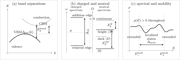
Three different operations can produce a reported gap. Left: a vertical transition keeps crystal momentum fixed, whereas the global band gap compares extrema at different momenta. Center: electron addition and removal define a charged continuum, while a neutral exciton can lie below it and optical selection can hide lower neutral states. Right: localized states can fill a spectral interval even though no extended states occur between two mobility edges.

Charged Excitations and Quasiparticle Edges

Band eigenvalues cease to be the primary definition when interactions are essential. Hold the external potential, nuclear geometry, boundary conditions, and other control parameters fixed, and let $E_0(N)$ be the exact ground-state energy with $N$ particles. Define the addition and removal chemical potentials

$$\mu^+(N) = E_0(N+1)-E_0(N)$$

and

$$\mu^-(N) = E_0(N)-E_0(N-1).$$

The full charge gap, also called the interacting fundamental gap, is

$$\begin{aligned} \Delta_{\mathrm{ch}} &= \mu^+(N)-\mu^-(N) \\ &= E_0(N+1)+E_0(N-1)-2E_0(N). \end{aligned}$$

With the conventional positive ionization energy $I=E_0(N-1)-E_0(N)$ and electron affinity $A=E_0(N)-E_0(N+1)$,

$$\Delta_{\mathrm{ch}}=I-A.$$

This is a thermodynamic particle-number difference. It is meaningful even when no single band labels the low-energy states. Some many-body literature uses $\Delta_c$ for half this quantity, especially under particle–hole symmetry. A numerical value without the full-gap or half-gap convention is incomplete.

For a noninteracting band insulator in the thermodynamic limit, $\Delta_{\mathrm{ch}}=E_g^{\mathrm{band}}$. Interactions can instead open a Mott charge gap, renormalize an existing band gap, or transfer edge weight into continua. The equality to a fixed-band separation is then not available. Martin, Reining, and Ceperley give a systematic many-body treatment of these particle-addition and removal energies.

Spectral gap versus quasiparticle gap

The zero-temperature one-particle spectral function has removal support at energies associated with transitions from $N$ to $N-1$ particles and addition support associated with transitions from $N$ to $N+1$. The absence of support around the chemical potential defines a one-particle spectral gap for the chosen operator and thermodynamic state.

A quasiparticle gap is more restrictive. It is the separation between the lowest coherent addition and removal poles, or between sufficiently narrow peaks that can be followed as quasiparticle bands. The Green-function framework introduced by Hedin and the semiconductor calculations of Hybertsen and Louie motivate the $GW$ approximation to such addition and removal energies. The review by Onida, Reining, and Rubio explains why the electron self-energy and the electron–hole response solve different excitation problems.

Three distinctions follow.

• A charge gap can exist even if the thresholds are broad continua and no long-lived quasiparticle is present.
• A sharp occupied removal edge alone does not determine the full gap; the addition edge is also required on the same energy reference.
• A computed $GW$ gap is a method-labelled approximation to quasiparticle energies. It is not, by its name alone, an exact charge gap or a measured optical onset.

Spectral Functions owns poles, residues, linewidths, continua, and the map from an intrinsic spectrum to a measured intensity.

Finite systems and charged supercells

For a finite isolated sample, $E_0(N\pm1)$ can include physical charging energy. In a periodic charged-cell calculation it can also include the chosen neutralizing background, image interactions, potential alignment, and finite-$\mathbf k$ sampling. In exact diagonalization, a level spacing or a shell effect can mimic a gap. A thermodynamic charge-gap claim therefore needs either a size extrapolation or a documented correction scheme appropriate to the geometry and electrostatics.

Do not relax the ions in one charge sector while holding them fixed in another unless an adiabatic or relaxed-ion gap is explicitly intended. A vertical electronic gap and a relaxed addition energy include different lattice physics.

Kohn–Sham Gaps and the Derivative Discontinuity

Kohn–Sham density-functional theory replaces the interacting ground-state problem by an auxiliary noninteracting system constructed to reproduce the ground-state density. Kohn and Sham derived the self-consistent auxiliary equations; the complete spectrum of their operator was not introduced as an exact spectrum of charged excitations.

For the exact multiplicative Kohn–Sham potential, define the global occupied–empty gap

$$\Delta_{\mathrm{KS}} = \varepsilon_{\mathrm{LUMO}}^{\mathrm{KS}} - \varepsilon_{\mathrm{HOMO}}^{\mathrm{KS}},$$

with the corresponding full-zone extrema in a periodic solid. Exact ground-state DFT gives the decomposition

$$\Delta_{\mathrm{ch}} = \Delta_{\mathrm{KS}} + \Delta_{\mathrm{xc}},$$

where $\Delta_{\mathrm{xc}}$ is the constant discontinuous shift of the exact exchange-correlation potential as the particle number crosses an integer. Perdew, Parr, Levy, and Balduz established the piecewise-linear energy and integer discontinuity; Perdew and Levy and, independently, Sham and Schlüter connected that discontinuity to the energy gap.

This exact relation is a warning about identification, not a universal recipe for correcting an approximate calculation.

What the decomposition does and does not say

• A Kohn–Sham gap is a well-defined eigenvalue separation of a declared auxiliary operator. It is not generally the exact charge gap.
• Common local and semilocal approximations do not reproduce the exact discontinuity and can have self-interaction, delocalization, and correlation errors. Nevertheless, “DFT always underestimates gaps” is not a theorem about every functional, material, geometry, or reported gap.
• Hybrid and other generalized Kohn–Sham methods use nonmultiplicative operators. Their eigenvalue gaps can absorb part of what appears as a discontinuity in multiplicative Kohn–Sham theory, so the simple equation above cannot be transferred term by term without defining the formalism.
• A scissor shift, tuned hybrid, Hubbard correction, or $GW$ calculation is a method and parameter choice. Agreement with one measured onset is not an independent validation if that onset was used to tune the correction.

Report the functional, magnetic state, spin–orbit treatment, structure, $\mathbf k$ search, convergence controls, and whether the value is a direct or global Kohn–Sham gap. Then compare it only with an observable whose excitation sector and forward model have also been declared.

Neutral and Optical Thresholds

A neutral excitation remains in the $N$-particle Hilbert space. Its absolute lowest threshold is

$$\Delta_{\mathrm{neutral}} = \min_{S\ne0} \left[ E_S(N)-E_0(N) \right].$$

The lowest neutral state may be a spin excitation, a dark exciton, a finite-momentum state, a collective mode, or a symmetry-forbidden transition. It need not appear in ordinary long-wavelength absorption.

For incident polarization $\hat{\mathbf e}$ and photon momentum negligible on the Brillouin-zone scale, an idealized optical threshold can be written

$$E_g^{\mathrm{opt}} = \inf_{ \langle S| \hat{\mathbf e}\!\cdot\!\hat{\mathbf j} |0\rangle\ne0 } \left[ E_S(N)-E_0(N) \right].$$

The operator, polarization, geometry, and assistance mechanism are part of the definition. In an indirect semiconductor, a phonon can supply the missing crystal momentum; the onset then contains both electronic and phonon energies and a temperature-dependent occupation factor. Elliott’s analysis remains the classic account of allowed and forbidden direct-transition exciton series and their continuum line shapes; an indirect phonon-assisted onset needs a separate electron–phonon response model.

Exciton binding is a difference between matched thresholds

Let $E_X$ be the excitation energy of a specified bound electron–hole state, measured from $E_0(N)$, and let $E_{\mathrm{cont}}$ be the free electron–hole continuum threshold in the same material, environment, momentum sector, geometry, and temperature. Its binding energy is

$$E_b^X = E_{\mathrm{cont}}-E_X.$$

When coherent quasiparticle edges define that continuum, one often writes

$$E_b^X = \Delta_{\mathrm{QP}}-E_X.$$

The familiar shorthand $E_g^{\mathrm{opt}}\simeq\Delta_{\mathrm{QP}}-E_b^X$ is valid only when $E_X$ is the lowest transition visible in the declared optical channel. The lowest exciton may be dark, spin forbidden, momentum indirect, or hidden by disorder and resolution. Conversely, an Urbach tail or defect transition can put weak absorption below the clean continuum without defining the intrinsic band gap.

Rohlfing and Louie show how quasiparticle energies and the electron–hole Bethe–Salpeter problem combine in a first-principles optical spectrum. This page retains only the threshold ledger; the internal exciton wavefunction, screening kernel, Rydberg series, and material taxonomy belong to the dedicated exciton treatment when it is promoted.

Absorption, emission, and photoemission are different records

• Absorption and ellipsometry constrain optically active neutral response after propagation, polarization, and line-shape modeling.
• Photoluminescence records radiative recombination after carriers and excitons have relaxed. Stokes shifts, localization, defects, and nonequilibrium populations can move its peak below an absorption edge.
• ARPES samples occupied removal spectral weight. It does not see the unoccupied addition edge needed for a full charge or quasiparticle gap.
• Inverse photoemission samples addition weight, but combining it with ARPES requires aligned energy zeros, compatible surfaces, and comparable state preparation.
• STS measures a tunneling-matrix-weighted local spectrum at a surface. Tip-induced band bending, charging, surface states, and the setpoint can move or obscure apparent edges.

Damascelli, Hussain, and Shen review the ARPES matrix-element and surface boundary; Tersoff and Hamann give the standard tunneling connection behind the STS qualification. The corresponding ARPES and STM/STS pages own the full experimental forward models.

Transport Activation and Mobility Gaps

Transport does not measure an energy spectrum without a kinetic model. If a conductivity is fitted to

$$\sigma(T) = \sigma_0(T) \exp\!\left( -\frac{E_A}{k_{\mathrm B}T} \right),$$

then $E_A$ is the activation energy of that fit. Its physical interpretation depends on the carrier source, chemical potential, mobility, contacts, temperature interval, and competing channels. A straight segment in an Arrhenius plot is evidence for an exponential scale, not by itself a band gap.

The intrinsic-semiconductor factor of two

For a clean, nondegenerate intrinsic semiconductor in equilibrium, let $E_g^{\mathrm{free}}(T)$ denote the thermally renormalized threshold for creating a free electron–hole pair. Then

$$n_i = \sqrt{N_cN_v} \exp\!\left( -\frac{E_g^{\mathrm{free}}(T)}{2k_{\mathrm B}T} \right),$$

and

$$\sigma = e \left( n\mu_e+p\mu_h \right).$$

If intrinsic carriers dominate and the effective densities of states and mobilities vary slowly compared with the exponential over the fit window, then

$$E_A \simeq \frac{E_g^{\mathrm{free}}(T)}{2}.$$

Sze and Ng and Yu and Cardona develop this semiconductor limit. Some authors report the fitted $E_A$; others call $2E_A$ the transport gap. The fit equation must accompany the number. Only when the free-carrier threshold is nearly temperature independent over the fit window and is matched to the interacting charge threshold may one further write $E_A\simeq\Delta_{\mathrm{ch}}/2$.

The factor of two fails when the chemical potential is pinned away from midgap, one carrier dominates, dopants are being ionized, contacts or grain boundaries control the resistance, polarons activate, parallel surface channels conduct, or the prefactor changes appreciably. A crossover between two channels can even imitate a limited Arrhenius window.

Mobility edges and localized spectral weight

In a one-particle disordered problem, a mobility edge separates localized from extended states in the thermodynamic limit. If two such edges bound an interval containing no extended states,

$$E_-^{\mathrm{mob}} < E < E_+^{\mathrm{mob}},$$

one may define the full mobility-gap width

$$\Delta_{\mathrm{mob}} = E_+^{\mathrm{mob}}-E_-^{\mathrm{mob}}.$$

The density of states can remain nonzero throughout this interval because the states are localized. If simple activation from a chemical potential inside the interval to the nearest extended state controls transport, the one-sided scale is

$$E_A^{\mathrm{edge}} = \min\!\left( E_+^{\mathrm{mob}}-\mu, \mu-E_-^{\mathrm{mob}} \right).$$

It is generally neither the full mobility gap nor half of it. Mott introduced the mobility-edge language for disordered structures; Anderson’s localization mechanism, the scaling theory of Abrahams and collaborators, and the review by Evers and Mirlin establish why dimension, symmetry class, size scaling, and wavefunction statistics matter.

Hopping among localized states can produce finite-temperature conduction even inside a mobility gap. Mott variable-range hopping has the idealized form

$$\sigma(T) \sim \exp\!\left[ -\left( \frac{T_0}{T} \right)^{1/(d+1)} \right],$$

while the Coulomb-gap analysis of Efros and Shklovskii gives exponent $1/2$ under its own assumptions. Neither law defines a hard spectral gap. Mobility Edges owns localization diagnostics and critical scaling; Anderson Insulators owns hopping transport and Coulomb-gap inference.

Methods and Probes by Gap Object

No method returns an unqualified “true band gap.” It returns an estimator or response tied to a Hamiltonian, operator, state, and approximation.

Computational access

Method	Native output	Gap it can support	Required qualification
tight-binding or model diagonalization	model eigenvalues and eigenvectors	direct and global model-band gaps	active orbitals, fitted range, symmetry, full-zone search
Kohn–Sham DFT	auxiliary eigenvalues and ground-state density	direct and global Kohn–Sham gaps	functional, generalized-KS status, structure, spin, convergence
total-energy differences or $\Delta$SCF	$E_0(N\pm1)-E_0(N)$ estimates	charge gap	fixed versus relaxed geometry, charged-cell corrections, size limit
$GW$ or another self-energy approximation	addition/removal quasiparticle energies	quasiparticle gap	starting point, self-consistency, screening, frequency and basis convergence
Bethe–Salpeter, configuration interaction, or qualified TDDFT	neutral excitation energies and oscillator strengths	neutral and optical gaps	kernel, active space, polarization, dark states, continuum convergence
exact diagonalization or tensor-network energy differences	finite-system many-body levels	charge and neutral gaps	boundary conditions, sector choice, truncation, finite-size scaling
transfer matrix, participation scaling, or conductance scaling	localization length or size-dependent transport	mobility edges and mobility gap	disorder ensemble, symmetry class, dimensions, thermodynamic scaling

The $GW$ and Bethe–Salpeter division in the table is conceptual rather than a software prescription: self-energy poles address charged one-particle excitations, whereas an electron–hole kernel addresses neutral response. Onida, Reining, and Rubio provide the standard comparison.

Experimental access

Probe	Closest native record	Gap inference	Principal ambiguity
ARPES	occupied momentum-resolved removal intensity	occupied edge or removal dispersion	no addition edge; matrix elements, surface, resolution
inverse photoemission	unoccupied addition intensity	addition edge	energy alignment, surface and resolution differ from ARPES
STS	local tunneling-weighted addition/removal spectrum	local spectral threshold	tip, surface, band bending, charging, in-gap states
optical absorption or ellipsometry	polarization-resolved neutral response	optically active threshold	excitons, phonons, forbidden transitions, tails, propagation
photoluminescence	relaxed radiative emission	recombination scale	Stokes shift, defects, population kinetics, dark reservoirs
dc transport versus temperature	conductivity or resistivity tensor	activation energy or hopping scale	prefactor, chemical potential, contacts, parallel channels
compressibility or capacitance	particle-number response	charge-addition threshold under a device model	electrostatics, geometry, disorder, reservoirs
thermally activated Hall or Corbino transport	bulk carrier response	distance to an extended-state threshold	mobility, disorder broadening, edge or surface channels

The strongest result combines complementary records. For example, ARPES plus inverse photoemission can bracket occupied and empty spectral weight; optical absorption can then expose the neutral electron–hole shift; transport can test whether carriers actually become mobile. Agreement is meaningful only after the specimen, temperature, strain, surface, doping, and energy references are matched.

Worked Gap Audits

Parallel bands with a positive direct gap and indirect overlap

Let $k\in[-\pi/a,\pi/a]$ and consider two noninteracting bands

$$\varepsilon_v(k) = -\frac{\Delta}{2} +2t\cos(ka)$$

and

$$\varepsilon_c(k) = +\frac{\Delta}{2} +2t\cos(ka),$$

with $t>0$ and $\Delta>0$. Their separation at every common momentum is

$$\varepsilon_c(k)-\varepsilon_v(k)=\Delta,$$

so

$$E_g^{\mathrm{dir}}=\Delta.$$

The valence maximum occurs at $k=0$, while the conduction minimum occurs at $k=\pi/a$. Therefore

$$E_g^{\mathrm{band}} = \left( \frac{\Delta}{2}-2t \right) - \left( -\frac{\Delta}{2}+2t \right) = \Delta-4t.$$

For $\Delta>4t$ the system has a positive indirect band gap. At $\Delta=4t$ the indirect gap closes. For $0<\Delta<4t$, every vertical separation remains positive, yet the energy ranges overlap and the nominal insulating filling produces electron and hole pockets. This simple example separates a direct projector gap from a global insulating gap.

One material, four reported numbers

Suppose a calculation reports

$$\Delta_{\mathrm{KS}}=1.4\,\mathrm{eV}, \qquad \Delta_{\mathrm{xc}}=0.6\,\mathrm{eV},$$

and a matched quasiparticle-plus-electron–hole calculation gives a bright exciton binding energy $E_b^X=0.25\,\mathrm{eV}$. Assume that the coherent quasiparticle continuum begins at the same threshold, $\Delta_{\mathrm{QP}}=\Delta_{\mathrm{ch}}$. Within this declared ledger,

$$\Delta_{\mathrm{ch}} \simeq 2.0\,\mathrm{eV}$$

and

$$E_X \simeq 1.75\,\mathrm{eV}.$$

If intrinsic conductivity has a fitted activation energy $E_A=0.92\,\mathrm{eV}$, it is tempting to double it and call $1.84\,\mathrm{eV}$ the same charge gap. That comparison is not yet licensed. One must verify intrinsic carrier balance, the mobility prefactor, chemical potential, contacts, and the fit interval. The four numbers are mutually compatible within plausible uncertainties, but they do not become identical by being close.

A finite density of states inside a mobility gap

Let a disordered three-dimensional model have localized states for $-0.4\,\mathrm{eV}<E<0.1\,\mathrm{eV}$ and extended states immediately outside, while its density of states remains nonzero throughout. The full mobility gap is $0.5\,\mathrm{eV}$. If $\mu=-0.05\,\mathrm{eV}$, simple activation to the nearer mobility edge costs

$$E_A^{\mathrm{edge}} = \min(0.15,0.35)\,\mathrm{eV} = 0.15\,\mathrm{eV}.$$

The spectral gap is zero, the mobility-gap width is $0.5\,\mathrm{eV}$, and the nearest-edge activation scale is $0.15\,\mathrm{eV}$. At lower temperature, hopping through localized states may replace this Arrhenius law. All three statements can be true simultaneously.

Reliability Checks and Canonical Handoffs

A gap claim is mature only when its limiting procedure and exclusions are visible.

Full-zone and subspace checks

Search the complete Brillouin zone rather than a presentation path. Include all bands and internal sectors that can enter the target window. Near an avoided crossing, confirm that band interpolation and band sorting follow the same physical subspace. A local orbital reordering or reopened gap is not itself a topological invariant; use Topological Phase Transitions for the full-zone closing and phase evidence.

Temperature and lattice checks

State whether the quoted value is at zero temperature, a frozen experimental structure, or a finite-temperature renormalized edge. Thermal expansion, electron–phonon coupling, zero-point motion, disorder, and phase transitions can all move the band and optical thresholds. Giustino reviews the first-principles electron–phonon contribution; the sign and size remain material and method dependent.

Finite-size and electrostatic checks

Distinguish a bulk gap from level spacing, confinement, charging energy, supercell image effects, and a boundary-state splitting. Record the order of limits in system size, temperature, frequency, and broadening. For a device, band bending, reservoirs, quantum capacitance, and contact electrostatics can shift an apparent threshold; the future semiconductor-device owner will retain the junction calculation, while this page retains only the gap labels.

Disorder and localization checks

Crystal momentum is not exact in a disordered sample. If an unfolded or effective-medium band picture is used, label it as such. A mobility edge needs wavefunction, conductance, or localization-length scaling, not merely a smooth density-of-states shoulder. Conversely, a spectral gap does not determine a finite-temperature resistance without carriers, scattering, geometry, and contacts.

Probe and energy-reference checks

Match bulk or surface sensitivity, specimen preparation, chemical potential, temperature, strain, field, and energy zero before subtracting two measured edges. Convolve theory with the instrument resolution and include the relevant matrix elements. A missing peak can be a dark state or a matrix-element zero; an apparent in-gap feature can be a defect, boundary state, charging event, or background subtraction artifact.

The canonical stopping rules are:

• hand exciton structure and binding kernels to the exciton owner;
• hand response functions and optical sum rules to Optical Conductivity and Dielectric Response when those routes are substantive;
• hand hopping and localization criticality to Anderson Insulators and Mobility Edges;
• hand band inversion and invariant changes to the topology chapter;
• hand interface offsets and self-consistent band bending to the semiconductor and heterostructure owners; and
• hand acquisition, calibration, and inversion to the relevant spectroscopy page.

Common Pitfalls

Calling a direct separation the band gap. A positive vertical separation can coexist with indirect overlap. Compute both the minimum direct and global separations over the full zone.

Calling a Kohn–Sham gap the experimental gap. It is an eigenvalue gap of a declared auxiliary operator. State the functional and formalism, then compare with the matching charge or neutral observable through an explicit model.

Calling every spectral edge a quasiparticle edge. A continuum threshold can be sharp without supporting a coherent pole. Report residue and linewidth, or use the less restrictive term spectral threshold.

Subtracting unrelated measurements to obtain an exciton binding energy. The continuum and exciton must refer to the same material, environment, momentum sector, temperature, and state. A photoluminescence peak and a different specimen’s Kohn–Sham gap do not form a controlled subtraction.

Reading an Arrhenius slope without its convention. State whether the fit is to $\sigma$ or $\rho$, whether the reported number is $E_A$ or $2E_A$, and which channel dominates the chosen temperature interval.

Equating a mobility gap with zero density of states. A mobility gap excludes extended states, not all states. Localized tail states can support tunneling, compressibility, or hopping while dc transport remains insulating in the zero-temperature limit.

Inferring a thermodynamic gap from one finite size. Boundary conditions, shell filling, charging, and topological edge hybridization can all create a finite level spacing. Extrapolate or supply a controlled finite-size bound.

Exercises

1. Direct separation without an insulating gap

At every $\mathbf k$, two band manifolds obey $\varepsilon_c^{\min}(\mathbf k)-\varepsilon_v^{\max}(\mathbf k) \ge 0.30\,\mathrm{eV}$. Their global extrema are $\min\varepsilon_c=0.10\,\mathrm{eV}$ and $\max\varepsilon_v=0.25\,\mathrm{eV}$. Find the lower bound on the minimum direct gap and the global band gap. Classify the energy overlap.

Solution

The stated pointwise inequality gives

$$E_g^{\mathrm{dir}} \ge 0.30\,\mathrm{eV}.$$

The global gap is

$$E_g^{\mathrm{band}} = 0.10\,\mathrm{eV} - 0.25\,\mathrm{eV} = -0.15\,\mathrm{eV}.$$

Thus the manifolds are directly separated at every momentum but overlap in energy by $0.15\,\mathrm{eV}$. At the corresponding filling this is an overlap-semimetal situation, not an insulator.

2. The many-body charge gap

A finite cluster has ground-state energies $E_0(N-1)=-97.8\,\mathrm{eV}$, $E_0(N)=-100.0\,\mathrm{eV}$, and $E_0(N+1)=-101.1\,\mathrm{eV}$. Compute $\mu^-$, $\mu^+$, and the full charge gap. What additional step is needed for a bulk claim?

Solution

The removal and addition chemical potentials are

$$\mu^- = E_0(N)-E_0(N-1) = -2.2\,\mathrm{eV}$$

and

$$\mu^+ = E_0(N+1)-E_0(N) = -1.1\,\mathrm{eV}.$$

Therefore

$$\Delta_{\mathrm{ch}} = \mu^+-\mu^- = 1.1\,\mathrm{eV}.$$

The signs of the individual chemical potentials depend on the energy zero; their difference does not. A bulk claim still requires size and boundary scaling or controlled corrections for charging and finite-cell effects.

3. Kohn–Sham and optical ledgers

An exact multiplicative Kohn–Sham description has $\Delta_{\mathrm{KS}}=1.1\,\mathrm{eV}$ and $\Delta_{\mathrm{xc}}=0.7\,\mathrm{eV}$. A bright exciton lies $0.2\,\mathrm{eV}$ below the matched quasiparticle continuum. Estimate the charge gap and bright optical threshold under these assumptions.

Solution

The exact DFT decomposition gives

$$\Delta_{\mathrm{ch}} = 1.1\,\mathrm{eV} + 0.7\,\mathrm{eV} = 1.8\,\mathrm{eV}.$$

If the coherent quasiparticle continuum begins at the same threshold and the specified exciton is the lowest optically active state, then

$$E_g^{\mathrm{opt}} = 1.8\,\mathrm{eV} - 0.2\,\mathrm{eV} = 1.6\,\mathrm{eV}.$$

The last step would fail for a mismatched continuum, dark lowest exciton, indirect transition without its phonon ledger, or different temperature and environment.

4. Intrinsic activation convention

Over a controlled temperature window an intrinsic semiconductor has $\sigma(T)\propto\exp[-0.38\,\mathrm{eV}/(k_{\mathrm B}T)]$. Assuming slowly varying mobilities and effective densities of states, estimate the free-carrier gap governing the fit. Under what additional condition may it be identified with the interacting charge gap? Give two reasons the estimate can fail.

Solution

In the stated intrinsic limit the fitted exponent is half the thermally renormalized free-carrier threshold, so

$$E_g^{\mathrm{free}}(T) \simeq 2E_A = 0.76\,\mathrm{eV}.$$

This may be called $\Delta_{\mathrm{ch}}$ only if temperature renormalization is negligible over the fit window and the free-carrier threshold has been matched to the same interacting addition/removal continuum. The inference can fail if dopant ionization, a contact barrier, hopping, or a parallel channel controls the resistance; if the chemical potential is not near its intrinsic position; or if the mobility prefactor varies strongly over the fit window. Any two of these invalidate the simple factor-of-two interpretation.

5. Mobility width and nearest-edge activation

Localized states occupy the interval from $E_-^{\mathrm{mob}}=-0.6\,\mathrm{eV}$ to $E_+^{\mathrm{mob}}=0.4\,\mathrm{eV}$, and $\mu=0.1\,\mathrm{eV}$. Find the full mobility gap and the nearest-edge activation scale. Does a nonzero density of states at $\mu$ contradict either answer?

Solution

The full interval has width

$$\Delta_{\mathrm{mob}} = 0.4-(-0.6) = 1.0\,\mathrm{eV}.$$

The distances from the chemical potential to the upper and lower mobility edges are $0.3\,\mathrm{eV}$ and $0.7\,\mathrm{eV}$, respectively. Thus

$$E_A^{\mathrm{edge}} = 0.3\,\mathrm{eV}.$$

A nonzero density of localized states at $\mu$ is compatible with both statements. The mobility gap excludes extended states, not spectral weight.

6. Route four measurements

A sample has (a) an occupied ARPES edge, (b) an unoccupied inverse-photoemission edge, (c) a polarized absorption onset, and (d) a low-temperature variable-range-hopping fit. State the most direct gap information supplied by each record and one qualification needed before comparing them.

Solution

ARPES supplies occupied removal weight; inverse photoemission supplies addition weight. After energy alignment and surface/state matching, the two can constrain a single-particle or quasiparticle gap. Polarized absorption supplies an optically allowed neutral threshold subject to excitons, selection rules, phonons, propagation, and resolution. Variable-range hopping supplies a localization-and-hopping scale, not a hard band or spectral gap. The sample state, temperature, energy zero, surface sensitivity, and model must be matched before any numerical subtraction or equality claim.

7. Design a full-zone gap check

A calculation reports a $40\,\mathrm{meV}$ gap on a conventional high-symmetry path. List a minimal set of checks needed before calling it a global bulk gap, and state where the claim should be routed if the gap closes and reopens under a tuning parameter.

Solution

At minimum, search a converged full Brillouin-zone mesh; include all relevant bands, spinor sectors, valleys, magnetic domains, and structures; test basis, $\mathbf k$-mesh, interpolation, and finite-cell convergence; state the functional or Hamiltonian, filling, temperature, field, and energy reference; and attach uncertainties to the valence and conduction extrema. If disorder is present, replace the naive crystal-momentum claim with a declared unfolded or localization analysis. A tuned closing and reopening is then routed to Topological Phase Transitions for the symmetry, invariant, and phase evidence; the closing alone does not establish topology.

References

• E. Abrahams, P. W. Anderson, D. C. Licciardello, and T. V. Ramakrishnan, “Scaling Theory of Localization: Absence of Quantum Diffusion in Two Dimensions,” Physical Review Letters 42, 673–676 (1979).
• P. W. Anderson, “Absence of Diffusion in Certain Random Lattices,” Physical Review 109, 1492–1505 (1958).
• N. W. Ashcroft and N. D. Mermin, Solid State Physics (Holt, Rinehart and Winston, 1976), Chapters 7–12 and 28.
• M. L. Cohen and S. G. Louie, Fundamentals of Condensed Matter Physics, Cambridge University Press (2016).
• A. Damascelli, Z. Hussain, and Z.-X. Shen, “Angle-Resolved Photoemission Studies of the Cuprate Superconductors,” Reviews of Modern Physics 75, 473–541 (2003).
• A. L. Efros and B. I. Shklovskii, “Coulomb Gap and Low Temperature Conductivity of Disordered Systems,” Journal of Physics C: Solid State Physics 8, L49–L51 (1975).
• R. J. Elliott, “Intensity of Optical Absorption by Excitons,” Physical Review 108, 1384–1389 (1957).
• F. Evers and A. D. Mirlin, “Anderson Transitions,” Reviews of Modern Physics 80, 1355–1417 (2008).
• F. Giustino, “Electron–Phonon Interactions from First Principles,” Reviews of Modern Physics 89, 015003 (2017).
• L. Hedin, “New Method for Calculating the One-Particle Green’s Function with Application to the Electron-Gas Problem,” Physical Review 139, A796–A823 (1965).
• M. S. Hybertsen and S. G. Louie, “Electron Correlation in Semiconductors and Insulators: Band Gaps and Quasiparticle Energies,” Physical Review B 34, 5390–5413 (1986).
• W. Kohn and L. J. Sham, “Self-Consistent Equations Including Exchange and Correlation Effects,” Physical Review 140, A1133–A1138 (1965).
• R. M. Martin, L. Reining, and D. M. Ceperley, Interacting Electrons: Theory and Computational Approaches, Cambridge University Press (2016).
• N. F. Mott, “Electrons in Disordered Structures,” Advances in Physics 16, 49–144 (1967).
• G. Onida, L. Reining, and A. Rubio, “Electronic Excitations: Density-Functional versus Many-Body Green’s-Function Approaches,” Reviews of Modern Physics 74, 601–659 (2002).
• J. P. Perdew and M. Levy, “Physical Content of the Exact Kohn–Sham Orbital Energies: Band Gaps and Derivative Discontinuities,” Physical Review Letters 51, 1884–1887 (1983).
• J. P. Perdew, R. G. Parr, M. Levy, and J. L. Balduz Jr., “Density-Functional Theory for Fractional Particle Number: Derivative Discontinuities of the Energy,” Physical Review Letters 49, 1691–1694 (1982).
• M. Rohlfing and S. G. Louie, “Electron-Hole Excitations and Optical Spectra from First Principles,” Physical Review B 62, 4927–4944 (2000).
• L. J. Sham and M. Schlüter, “Density-Functional Theory of the Energy Gap,” Physical Review Letters 51, 1888–1891 (1983).
• S. M. Sze and K. K. Ng, Physics of Semiconductor Devices, 3rd ed., Wiley (2007).
• J. Tersoff and D. R. Hamann, “Theory of the Scanning Tunneling Microscope,” Physical Review B 31, 805–813 (1985).
• P. Y. Yu and M. Cardona, Fundamentals of Semiconductors: Physics and Materials Properties, 4th ed., Springer (2010).