Effective Mass

Effective mass is a local response coefficient extracted from the dispersion of a band or quasiparticle. It tells how band velocity changes when crystal momentum changes. Near a smooth band extremum, this response makes a Bloch electron behave approximately like a free particle with a modified, generally anisotropic mass:

$$\varepsilon_n(\mathbf k_0+\mathbf q) \approx \varepsilon_n(\mathbf k_0) + \frac{\hbar^2}{2} \mathbf q^{\mathsf T} \mathsf M_n^{-1} \mathbf q.$$

The tensor $\mathsf M_n$ is not the electron’s bare mass $m_e$. It summarizes the combined effect of kinetic energy, the periodic potential, orbital hybridization, and, when a quasiparticle dispersion is used, interaction renormalization. Its value depends on the band, expansion point, direction, energy window, and observable.

This page is the canonical home for the physical interpretation and derivation of effective mass in quantum matter. The Effective Mass formula card remains the compact lookup. Band Theory Overview owns the broader construction and interpretation of bands, while Fermi Surface owns constant-energy geometry and quantum-oscillation orbits.

Use the Band Theory and Electronic Structure gateway when you need to choose between classification, gap, carrier, dynamics, or response routes before committing to a mass approximation.

Required background. Band Theory Overview supplies smooth band dispersions, band indices, occupations, and the band-versus-quasiparticle distinction used here.

Helpful background. Density of States supplies spectral state counting, while Fermi Surface supplies constant-energy geometry and closed-orbit language.

Why a Crystal Can Change Inertia

For a free electron,

$$\varepsilon(\mathbf k) = \frac{\hbar^2 k^2}{2m_e},$$

so the curvature is fixed by $m_e$. In a crystal, Bragg scattering and orbital mixing reshape the dispersion. A broad band has large curvature and a light effective mass; a flat band has small curvature and a heavy mass. Curvature can even change sign within one band.

The crystal does not literally alter the rest mass or charge of the electron. Instead, an external force changes the electron’s crystal momentum, while the periodic lattice continually redistributes momentum between the wave packet and the crystal. Effective mass packages the resulting acceleration into a free-particle-like law over a limited region of momentum space.

Several quantities are called an effective mass:

Name	Defined by	Most directly relevant to
curvature tensor	Hessian of $\varepsilon_n(\mathbf k)$	local acceleration in a smooth band
density-of-states mass	state-counting equivalence	carrier density and thermodynamics
conductivity mass	current response with a scattering model	dc transport and mobility
cyclotron mass	energy derivative of orbit area	quantum oscillations and cyclotron resonance
optical mass	intraband spectral weight	Drude response and plasma frequency
quasiparticle mass	curvature or velocity of an interacting pole	low-energy interacting excitations

These masses coincide for a single isotropic parabolic band with energy-independent scattering. Outside that special case, a quoted value without a definition is incomplete.

Local Expansion of a Band

Let $\mathbf k_0$ be a point in a smooth, nondegenerate band and write

$$\mathbf q = \mathbf k-\mathbf k_0.$$

The Taylor expansion is

$$\begin{aligned} \varepsilon_n(\mathbf k_0+\mathbf q) ={}& \varepsilon_{n0} + \hbar\, \mathbf v_{n0}\cdot\mathbf q \\ &+ \frac{\hbar^2}{2} \sum_{ij} q_i \left( \mathsf M_n^{-1} \right)_{ij} q_j + O(q^3), \end{aligned}$$

where

$$\mathbf v_{n0} = \frac{1}{\hbar} \nabla_{\mathbf k} \varepsilon_n(\mathbf k) \biggr\rvert_{\mathbf k_0}$$

and

$$\left( \mathsf M_n^{-1} \right)_{ij} = \frac{1}{\hbar^2} \frac{\partial^2\varepsilon_n} {\partial k_i\,\partial k_j} \biggr\rvert_{\mathbf k_0}.$$

It is the inverse mass tensor that is directly equal to the Hessian divided by $\hbar^2$. The Hessian is real and symmetric for a smooth real-valued band energy, so it can be diagonalized by an orthogonal change of axes.

At a band extremum, $\mathbf v_{n0}=0$, and the quadratic term is the leading momentum dependence. Away from an extremum, the linear term must be retained. Silently dropping it changes both the reference velocity and the physical meaning of the approximation.

One dimension

In one dimension,

$$\frac{1}{m^*(k_0)} = \frac{1}{\hbar^2} \frac{d^2\varepsilon}{dk^2} \biggr\rvert_{k_0},$$

or

$$m^*(k_0) = \frac{\hbar^2} {d^2\varepsilon/dk^2\rvert_{k_0}}.$$

Positive curvature gives positive electron effective mass. Negative curvature gives negative electron effective mass. At an inflection point the inverse mass vanishes; writing $m^*=\infty$ is a shorthand for zero local acceleration under a force, not evidence that the wave packet has acquired infinite rest energy.

Principal masses

In principal-axis coordinates,

$$\mathsf M^{-1} = \operatorname{diag} \left( \frac{1}{m_1}, \frac{1}{m_2}, \frac{1}{m_3} \right).$$

A local minimum has $m_i>0$ in every direction. A local maximum has $m_i<0$ in the electron description. A saddle has mixed signs. At a degenerate critical point or band crossing, an individual-band Hessian can fail to be smooth or basis independent; a multiband effective Hamiltonian is then the correct object.

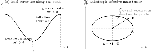
Effective mass is local and tensorial. In (a), one band contains positive, zero, and negative curvature. In (b), $\mathbf a=\mathsf M^{-1}\mathbf F$ need not be parallel to $\mathbf F$ when the principal masses differ.

Semiclassical Acceleration

The group velocity of a wave packet in band $n$ is

$$v_i = \frac{1}{\hbar} \frac{\partial\varepsilon_n} {\partial k_i}.$$

If a slowly varying perturbation produces a semiclassical force

$$\hbar\dot{\mathbf k} = \mathbf F,$$

then the chain rule gives

$$\begin{aligned} \dot v_i &= \frac{1}{\hbar} \sum_j \frac{\partial^2\varepsilon_n} {\partial k_i\,\partial k_j} \dot k_j \\ &= \sum_j \left( \mathsf M_n^{-1} \right)_{ij} F_j. \end{aligned}$$

Thus

$$\dot{\mathbf v} = \mathsf M_n^{-1}\mathbf F.$$

This is the dynamical origin of the curvature mass. If $\mathsf M$ is anisotropic, force and acceleration need not be parallel. For an electron of charge $-e$ in electric and magnetic fields, the ordinary band-force term is

$$\mathbf F = -e \left( \mathbf E+\mathbf v\times\mathbf B \right).$$

The derivation assumes a wave packet confined to one smooth band and fields varying slowly on microscopic scales. Semiclassical Dynamics of Bloch Electrons owns that packet construction, the signed electric- and magnetic-field force law, trajectories, and the tests for interband or quantized breakdown. Berry curvature can add an anomalous velocity, magnetic moments can shift the energy, and strong fields can drive interband tunneling. Those effects are corrections to the simple acceleration law, not alternative definitions of the Hessian retained here.

What the Tensor Means

Consider an ellipsoidal conduction-band minimum:

$$\varepsilon(\mathbf k_0+\mathbf q) = E_c + \frac{\hbar^2}{2} \left( \frac{q_1^2}{m_1} + \frac{q_2^2}{m_2} + \frac{q_3^2}{m_3} \right).$$

Constant-energy surfaces are ellipsoids. Along principal axis $i$,

$$v_i = \frac{\hbar q_i}{m_i}, \qquad \dot v_i = \frac{F_i}{m_i}.$$

If the force is not along a principal axis, each component is rescaled differently. A scalar mass is therefore meaningful only after specifying a direction, symmetry average, or measurement.

Symmetry constraints

Crystal symmetry constrains the tensor at high-symmetry points:

• cubic symmetry forces a nondegenerate extremum to have $\mathsf M=m^*\mathsf I$;
• uniaxial symmetry permits longitudinal and transverse masses;
• lower symmetry permits three distinct principal masses and rotated principal axes;
• symmetry-protected degeneracy generally requires a matrix-valued multiband Hamiltonian rather than one scalar dispersion.

The tensor transforms under a spatial rotation $\mathsf R$ as

$$\mathsf M^{-1} \longmapsto \mathsf R \mathsf M^{-1} \mathsf R^{\mathsf T}.$$

Its eigenvalues are coordinate independent, but its displayed components are not.

Band Mixing and the k·p View

The curvature of a band is not determined only by the bare kinetic term. For a local periodic potential and an isolated nondegenerate band, perturbation theory for the cell-periodic Hamiltonian gives a representative $k\cdot p$ expression,

$$\begin{aligned} \left( \mathsf M_n^{-1} \right)_{ij} ={}& \frac{\delta_{ij}}{m_e} \\ &+ \frac{2}{m_e^2} \sum_{m\ne n} \frac{ \operatorname{Re} \left[ \langle n|p_i|m\rangle \langle m|p_j|n\rangle \right] }{ \varepsilon_n-\varepsilon_m }. \end{aligned}$$

The states and matrix elements are evaluated at the expansion point, with the momentum operator generalized as required away from $\mathbf k=0$. Remote bands alter the curvature through virtual mixing. Nearby bands usually produce the strongest renormalization because their energy denominators are small.

This formula explains why effective masses can be much lighter or heavier than $m_e$, why signs can differ between conduction and valence bands, and why narrow gaps often accompany strong nonparabolicity. It also exposes a danger: when two bands become degenerate, nondegenerate perturbation theory is singular. One must retain the coupled subspace and construct a multiband effective Hamiltonian.

Spin–orbit coupling, nonlocal pseudopotentials, and many-body self-energies modify the velocity matrix elements or the effective Hamiltonian. The displayed equation is a structural guide, not a universal computational formula for every electronic-structure method.

Electrons and Holes

Near a valence-band maximum $\mathbf k_v$, write

$$\varepsilon_v(\mathbf k_v+\mathbf q) \approx E_v - \frac{\hbar^2}{2} \mathbf q^{\mathsf T} \mathsf M_h^{-1} \mathbf q,$$

where $\mathsf M_h$ is positive definite. The electron curvature tensor at the maximum is negative:

$$\mathsf M_{e,v}^{-1} = -\mathsf M_h^{-1}.$$

A nearly full valence band is more simply described by its missing electrons. A hole carries charge $+e$, positive excitation energy measured downward from the valence maximum, and positive hole mass $\mathsf M_h$. This change of variables converts the collective response of many occupied negative-curvature electron states into the motion of a small number of positive carriers.

Negative electron effective mass does not mean negative rest mass, negative kinetic energy, or motion opposite to velocity. It means that the electron-band acceleration produced by a force has the opposite sign locally. Holes owns the filled-reference operator transformation, charge and state count, and momentum–velocity–current conventions; the curvature-sign derivation is the part retained here.

Density-of-States Mass

For the three-dimensional ellipsoidal minimum above, rescale momenta by

$$Q_i = \frac{q_i}{\sqrt{m_i}}.$$

The energy becomes spherical in $\mathbf Q$ space, while the volume element acquires the Jacobian

$$d^3q = \sqrt{m_1m_2m_3}\, d^3Q.$$

Define the three-dimensional density-of-states mass by

$$m_{\mathrm{DOS}} = \left( m_1m_2m_3 \right)^{1/3}.$$

For total degeneracy $g$, including only degeneracies not already counted as separate bands, the density of states per physical volume is

$$\rho(E) = \frac{g}{4\pi^2} \left( \frac{2m_{\mathrm{DOS}}}{\hbar^2} \right)^{3/2} \sqrt{E-E_c}\, \Theta(E-E_c).$$

In two dimensions,

$$m_{\mathrm{DOS}}^{(2D)} = \sqrt{m_1m_2},$$

and the parabolic-band density of states is constant:

$$\rho_{2D}(E) = \frac{g\,m_{\mathrm{DOS}}^{(2D)}} {2\pi\hbar^2} \Theta(E-E_c).$$

The geometric mean appears because density of states counts momentum-space volume. Valley multiplicity is a separate factor. Folding a degeneracy into both $g$ and $m_{\mathrm{DOS}}$ double counts states.

The Density of States page develops normalization, dimensional threshold laws, van Hove singularities, projected densities, and numerical methods.

Conductivity Mass

In a one-valley parabolic model with a scalar, momentum-independent relaxation time $\tau$, the Drude conductivity tensor is

$$\boldsymbol{\sigma} = nq^2\tau\, \mathsf M^{-1}.$$

Drude Theory owns the relaxation equation, dc and optical conductivity, Hall tensor, lifetime distinctions, and experimental fitting tests. Here the equation serves only to define the conductivity-mass reduction.

Along a unit vector $\hat{\mathbf n}$, define

$$\frac{1} {m_{\mathrm{cond}}(\hat{\mathbf n})} = \hat{\mathbf n}^{\mathsf T} \mathsf M^{-1} \hat{\mathbf n}.$$

In principal axes,

$$\sigma_{ii} = \frac{nq^2\tau}{m_i}.$$

For equally populated equivalent valleys in a cubic material, each with one longitudinal mass $m_l$ and two transverse masses $m_t$, the orientationally averaged conductivity mass is

$$m_{\mathrm{cond}} = \frac{3} {m_l^{-1}+2m_t^{-1}}.$$

This harmonic-type average differs from the density-of-states mass. In a real multiband material, the conductivity also weights velocities, lifetimes, carrier densities, and scattering anisotropy over the Fermi surface. A mobility measurement gives $\mu=|q|\tau/m_{\mathrm{cond}}$ only within a specified scattering model; it cannot determine mass without information about $\tau$.

Cyclotron Mass

In a magnetic field, a semiclassical orbit follows the intersection of a constant-energy surface with a plane perpendicular to $\mathbf B$. Let $A(E,k_\parallel)$ be the enclosed $k$-space area at fixed momentum component along the field. The positive cyclotron-mass magnitude extracted from temperature damping is

$$m_c = \frac{\hbar^2}{2\pi} \left\lvert \frac{\partial A}{\partial E} \right\rvert_{k_\parallel}.$$

The magnitude of this derivative controls the temperature damping measured in Quantum Oscillations through the Lifshitz–Kosevich factor. A signed orbital mass can be retained separately to encode electron-like or hole-like circulation, but the Lifshitz–Kosevich mass quoted from damping is positive. It is therefore an orbit property, not simply one Cartesian component of the curvature tensor.

For a parabolic ellipsoid with $\mathbf B$ along principal axis $3$,

$$m_c = \sqrt{m_1m_2}.$$

More generally, for a positive mass tensor and field direction $\hat{\mathbf n}$,

$$m_c(\hat{\mathbf n}) = \sqrt{ \frac{\det\mathsf M} {\hat{\mathbf n}^{\mathsf T} \mathsf M \hat{\mathbf n}} }.$$

The formula applies to a central orbit of a parabolic ellipsoid. For a general Fermi surface, one must calculate the actual orbit area and its energy derivative. Multiple extremal orbits can produce several measured masses even within one band. Landau Levels in Solids takes a declared local mass tensor as an input and owns the resolved material-band ladder, including anisotropy, Zeeman and orbital terms, valley structure, and the field window in which the quadratic reduction remains controlled.

Optical and Plasma Masses

For an ideal parabolic carrier gas,

$$\left( \boldsymbol{\omega}_{p}^{\,2} \right)_{ij} = \frac{nq^2}{\epsilon_0} \left( \mathsf M^{-1} \right)_{ij}.$$

The intraband optical spectral weight therefore defines an optical or Drude mass. In a lattice, that weight is an occupation-weighted average of band curvature or Fermi-surface velocities, and interband transitions redistribute spectral weight. The total continuum $f$-sum rule involves the bare electron mass, while a low-frequency partial sum can involve a band or quasiparticle mass. Confusing the partial Drude weight with the full sum rule is a common source of apparently contradictory masses.

Interacting Quasiparticle Mass

Band calculations provide a reference dispersion $\varepsilon_b(\mathbf k)$. Interactions dress it through a self-energy $\Sigma(\mathbf k,\omega)$. Near a coherent Fermi-surface point, the quasiparticle residue is

$$Z = \left[ 1 - \frac{\partial \operatorname{Re}\Sigma} {\partial\omega} \right]^{-1}_{\mathrm F},$$

when $\omega$ is measured in energy units. The renormalized Fermi velocity is

$$\mathbf v_{\mathrm F}^{*} = Z \left[ \mathbf v_b + \frac{1}{\hbar} \nabla_{\mathbf k} \operatorname{Re}\Sigma \right]_{\mathrm F}.$$

An isotropic velocity mass can then be defined by

$$m_v^* = \frac{\hbar k_{\mathrm F}} {v_{\mathrm F}^{*}}.$$

This need not equal a simple Hessian mass away from a parabolic extremum. The specific-heat mass weights the interacting density of states; quantum oscillations measure an orbit mass; optical and dc responses can include vertex corrections and backflow. In a Galilean-invariant fluid, interactions can strongly renormalize the quasiparticle mass while conservation laws constrain the uniform current response.

The Fermi Liquid Theory Preview is the canonical home for quasiparticle residue, self-energy renormalization, Landau parameters, backflow, and thermodynamic mass. Polarons Preview treats mass enhancement from a particle dragging a deformable environmental cloud.

Worked Band Examples

One-dimensional cosine band

For nearest-neighbor hopping,

$$\varepsilon(k) = -2t\cos(ka),$$

the velocity and inverse mass are

$$v(k) = \frac{2ta}{\hbar} \sin(ka),$$ $$\frac{1}{m^*(k)} = \frac{2ta^2}{\hbar^2} \cos(ka).$$

Near $k=0$ the mass is positive:

$$m^*(0) = \frac{\hbar^2}{2ta^2}.$$

Near $k=\pi/a$ it is negative in the electron description. At $ka=\pi/2$, the inverse mass vanishes while the speed is maximal. A single constant $m^*$ cannot represent the whole band.

Nonparabolic semiconductor band

A common two-band approximation is

$$E(1+\alpha E) = \frac{\hbar^2k^2} {2m_{\mathrm{edge}}},$$

where $E$ is measured from the band edge. The isotropic cyclotron or velocity mass becomes

$$m_c(E) = m_{\mathrm{edge}} \left( 1+2\alpha E \right).$$

The carrier becomes heavier as energy increases when $\alpha>0$. A parabolic fit therefore depends on the fitted energy window. The local curvature mass, velocity mass, and cyclotron mass need not remain identical once nonparabolicity is appreciable.

Dirac cone

For an isotropic cone,

$$\varepsilon_{\pm}(k) = \pm\hbar v_D k,$$

there is no constant band-edge curvature mass. Nevertheless, a circular orbit at energy $E$ has

$$A(E) = \pi \left( \frac{E}{\hbar v_D} \right)^2,$$

and hence

$$m_c(E) = \frac{|E|}{v_D^2}.$$

The finite, density-dependent cyclotron mass does not contradict the vanishing radial second derivative of a linear dispersion. The two definitions probe different derivatives.

Extracting a Mass from Data

From a numerical band

If the curvature in one direction is reported as

$$C = \frac{d^2E}{dk^2}$$

in units of $\mathrm{eV\,\mathring A^2}$, then

$$\frac{m^*}{m_e} \approx \frac{7.62}{C}.$$

The sign of $C$ must be retained. If a fit is written as

$$E(k) = E_0 + A(k-k_0)^2,$$

then $C=2A$ and

$$\frac{m^*}{m_e} \approx \frac{3.81}{A},$$

with $A$ in $\mathrm{eV\,\mathring A^2}$.

For a tensor fit:

1. choose a physically justified expansion point and energy window;
2. express all components of $\mathbf k$ in the same reciprocal-length units;
3. fit the full symmetric quadratic form, including cross terms;
4. symmetrize the numerical Hessian;
5. diagonalize it and report principal axes as well as eigenvalues;
6. repeat the fit over several windows to expose nonparabolicity and numerical noise.

A polynomial can always return a number. Stability under reasonable changes of window is part of the evidence that the number represents an effective mass.

From experiment

• ARPES measures a spectral dispersion and can infer local velocities or curvature. Resolution, matrix elements, surface sensitivity, and self-energy structure affect the fit.
• Quantum oscillations determine extremal orbit areas from frequencies and cyclotron masses from temperature damping. The result is orbit specific.
• Cyclotron resonance probes the dynamical orbit mass and can separate carrier types under favorable conditions.
• Specific heat weights the quasiparticle density of states near the chemical potential and often yields a thermodynamic mass enhancement.
• Optical conductivity constrains intraband spectral weight and scattering rate, permitting a Drude mass only with a carrier-density and multiband model.
• Transport measures combinations of carrier density, velocity, lifetime, and mass. Hall data do not generally return an effective mass directly.

Different well-performed experiments can therefore report different masses without disagreement. The comparison is meaningful only after matching the band, orbit, direction, energy, temperature, and response definition.

Where the Approximation Breaks Down

The constant effective-mass approximation is reliable when:

• the relevant band is smooth and isolated over the occupied wave-packet region;
• the momentum or energy window is small enough that cubic and higher terms are negligible;
• the wave packet remains in one band under the applied fields;
• the fields vary slowly compared with lattice scales;
• the quasiparticle peak is sufficiently coherent if interactions are present;
• the chosen tensor or scalar matches the response being modeled.

It becomes unreliable or ambiguous in several important regimes.

Crossings and near-degeneracies

At an exact crossing, an individual eigenvalue can be nonanalytic and an individual eigenvector is basis dependent inside the degenerate subspace. Near an avoided crossing, curvature can vary rapidly. A multiband $k\cdot p$ model is usually more faithful than fitting one branch to a parabola.

Saddles and van Hove points

A saddle has positive curvature in some directions and negative curvature in others. Its mass tensor is indefinite, and a scalar average can conceal the geometry responsible for a van Hove singularity.

Inflection points

At an inflection point one principal inverse mass vanishes. Higher derivatives control the dynamics in that direction. Treating the divergent scalar mass as a globally heavy particle misses the finite velocity and rapid variation nearby.

Strong fields and interband motion

If a field moves the packet through a significant fraction of the Brillouin zone, the local tensor changes along the trajectory. Near small gaps, Landau–Zener transitions invalidate one-band dynamics. Magnetic fields strong enough to quantize motion require Landau-level or magnetic-breakdown descriptions.

Geometric corrections

Berry curvature produces an anomalous velocity transverse to the applied force, even without an off-diagonal mass tensor. Orbital magnetic moments shift the band energy in a field. These geometric effects should not be absorbed into an invented scalar mass.

Incoherent or strongly reconstructed spectra

If no sharp quasiparticle pole exists, assigning a band curvature to a broad spectral feature can be misleading. Symmetry breaking, strong correlations, disorder, or coupling to collective modes can also reconstruct the low-energy dispersion and make the mass temperature, field, or frequency dependent.

Common Mistakes

• Calling $m^*$ a material constant without naming the band, momentum, direction, and observable.
• Confusing the bare electron mass $m_e$ with a band or quasiparticle mass.
• Dropping the linear term when expanding away from a band extremum.
• Inverting each Hessian component separately instead of inverting or diagonalizing the full tensor.
• Replacing anisotropic masses by an arithmetic average regardless of the response.
• Interpreting negative curvature as negative rest mass or negative kinetic energy.
• Double counting spin or valley degeneracy in a density-of-states mass.
• Inferring mass directly from mobility without an independent scattering time.
• Equating a Dirac-band curvature, cyclotron mass, and density-of-states mass.
• Fitting across a crossing, saddle, or broad energy interval and reporting the result without a stability test.

A Reporting Checklist

A trustworthy mass statement answers six questions:

1. Which carrier, band, valley, or orbit is being described?
2. At what $\mathbf k$, energy, density, temperature, and field?
3. Is the quantity a tensor, a principal value, or an averaged scalar?
4. Is it a curvature, density-of-states, conductivity, cyclotron, optical, or thermodynamic mass?
5. Does it refer to a bare band calculation or an interacting quasiparticle?
6. Over what fitting window or model assumptions is it stable?

Writing $m^*=0.2m_e$ without this ledger is often not enough to reproduce or interpret the result.

Exercises

1. Curvature through a cosine band

For $\varepsilon(k)=-2t\cos(ka)$ with $t>0$, find the effective mass at $k=0$, $k=\pi/(2a)$, and $k=\pi/a$. Explain what happens at the middle point.

Solution

Differentiate twice:

$$\frac{d^2\varepsilon}{dk^2} = 2ta^2\cos(ka).$$

Therefore

$$m^*(k) = \frac{\hbar^2} {2ta^2\cos(ka)}.$$

At the band bottom,

$$m^*(0) = \frac{\hbar^2}{2ta^2}>0.$$

At $k=\pi/(2a)$, the curvature and inverse mass vanish. The effective mass is formally divergent, but the velocity

$$v = \frac{2ta}{\hbar}$$

is finite and maximal. The quadratic approximation fails because the leading change in velocity is controlled by higher derivatives. At the band top,

$$m^*(\pi/a) = -\frac{\hbar^2}{2ta^2}.$$

2. Force and acceleration in an anisotropic band

Let $\mathsf M=\operatorname{diag}(m,4m)$ and apply $\mathbf F=F(1,1)/\sqrt{2}$. Find $\mathbf a$ and determine whether it is parallel to $\mathbf F$.

Solution

The inverse tensor is

$$\mathsf M^{-1} = \frac{1}{m} \operatorname{diag} \left( 1,\frac{1}{4} \right).$$

Hence

$$\mathbf a = \mathsf M^{-1}\mathbf F = \frac{F}{\sqrt{2}m} \left( 1,\frac{1}{4} \right).$$

The force points at $45^\circ$, while the acceleration obeys

$$\tan\theta_a = \frac{a_y}{a_x} = \frac{1}{4}.$$

Thus $\theta_a\approx14.0^\circ$, and the vectors are not parallel.

3. Density-of-states mass of an ellipsoid

For principal masses $m_1=m$, $m_2=2m$, and $m_3=8m$, find the three-dimensional density-of-states mass. If there are six equivalent valleys and spin degeneracy remains unresolved, what total degeneracy multiplies the one-valley, one-spin density of states?

Solution

The density-of-states mass is

$$\begin{aligned} m_{\mathrm{DOS}} &= \left( m_1m_2m_3 \right)^{1/3} \\ &= \left( 16m^3 \right)^{1/3} \\ &= 16^{1/3}m \approx 2.52m. \end{aligned}$$

Six valleys and two spin states give

$$g = 6\times2 = 12.$$

The factor $12$ is kept separate from $m_{\mathrm{DOS}}$.

4. Cyclotron mass of a parabolic ellipsoid

For

$$E = \frac{\hbar^2}{2} \left( \frac{k_x^2}{m_x} + \frac{k_y^2}{m_y} + \frac{k_z^2}{m_z} \right),$$

take $\mathbf B\parallel\hat{\mathbf z}$ and the central orbit $k_z=0$. Derive $m_c$.

Solution

At fixed energy, the semiaxes of the orbit are

$$k_{x,\max} = \frac{\sqrt{2m_xE}}{\hbar}, \qquad k_{y,\max} = \frac{\sqrt{2m_yE}}{\hbar}.$$

Its area is

$$A(E) = \pi k_{x,\max}k_{y,\max} = \frac{2\pi E}{\hbar^2} \sqrt{m_xm_y}.$$

Therefore

$$\begin{aligned} m_c &= \frac{\hbar^2}{2\pi} \frac{\partial A}{\partial E} \\ &= \sqrt{m_xm_y}. \end{aligned}$$

The mass along the field, $m_z$, does not enter this central orbit.

5. Nonparabolic mass

Starting from

$$E(1+\alpha E) = \frac{\hbar^2k^2}{2m_{\mathrm{edge}}},$$

show that the isotropic cyclotron mass is $m_c(E)=m_{\mathrm{edge}}(1+2\alpha E)$.

Solution

The orbit area is

$$A(E) = \pi k^2 = \frac{2\pi m_{\mathrm{edge}}}{\hbar^2} E(1+\alpha E).$$

Using the orbit definition,

$$\begin{aligned} m_c(E) &= \frac{\hbar^2}{2\pi} \frac{\partial A}{\partial E} \\ &= m_{\mathrm{edge}} \left( 1+2\alpha E \right). \end{aligned}$$

Thus a finite-energy measurement need not recover the band-edge mass.

6. Converting a fitted curvature

A calculated conduction band is fitted near its minimum by

$$E(k) = E_c + 12.0\, \mathrm{eV\,\mathring A^2} \left( k-k_0 \right)^2.$$

Estimate $m^*/m_e$.

Solution

The coefficient is $A=12.0\,\mathrm{eV\,\mathring A^2}$, so

$$\frac{m^*}{m_e} \approx \frac{3.81}{A} = \frac{3.81}{12.0} \approx 0.318.$$

Equivalently, the curvature is $C=2A=24.0\,\mathrm{eV\,\mathring A^2}$ and $7.62/C$ gives the same result.

7. Apparently inconsistent measurements

An ARPES fit gives $0.7m_e$, quantum oscillations give $1.1m_e$, and a Drude analysis gives $0.5m_e$ for a multiband metal. Does this establish an experimental contradiction? List four checks needed before comparing the numbers.

Solution

No. The three probes do not automatically measure the same effective mass. One should check at least:

1. whether ARPES, the oscillation orbit, and the Drude response refer to the same band and Fermi-surface sheet;
2. whether the reported directions and magnetic-field orientations match;
3. whether temperatures, carrier densities, and reconstruction by an ordered phase are comparable;
4. whether the ARPES number is a local velocity or curvature mass, the oscillation number is an orbit mass, and the optical number depends on a multiband spectral-weight model;
5. whether interaction renormalization, surface sensitivity, unresolved valleys, or anisotropic scattering affect the probes differently.

Only after translating the measurements to a common carrier, geometry, and response definition is a numerical disagreement physically diagnostic.

References

• N. W. Ashcroft and N. D. Mermin, Solid State Physics, Holt, Rinehart and Winston, 1976.
• E. O. Kane, “Band Structure of Indium Antimonide,” Journal of Physics and Chemistry of Solids 1, 249–261 (1957), doi:10.1016/0022-3697(57)90013-6.
• C. Kittel, Introduction to Solid State Physics, 8th ed., Wiley, 2004.
• W. Kohn, “Effective Mass Theory in Solids from a Many-Particle Standpoint,” Physical Review 105, 509–517 (1957), doi:10.1103/PhysRev.105.509.
• J. M. Luttinger and W. Kohn, “Motion of Electrons and Holes in Perturbed Periodic Fields,” Physical Review 97, 869–883 (1955), doi:10.1103/PhysRev.97.869.
• M. P. Marder, Condensed Matter Physics, 2nd ed., Wiley, 2010.
• L. Onsager, “Interpretation of the de Haas–van Alphen Effect,” Philosophical Magazine 43, 1006–1008 (1952), doi:10.1080/14786440908521019.
• D. Shoenberg, Magnetic Oscillations in Metals, Cambridge University Press, 1984, doi:10.1017/CBO9780511897870.
• P. Y. Yu and M. Cardona, Fundamentals of Semiconductors, 4th ed., Springer, 2010, doi:10.1007/978-3-642-00710-1.