Landau Levels in Solids

Landau levels in a solid are the discrete magnetic-field eigenvalues of a declared low-energy band Hamiltonian, not automatically the free-electron ladder with the bare electron mass. A locally parabolic, nondegenerate band does inherit the canonical orbital spectrum after its curvature tensor is coupled to a uniform magnetic field. The spacing then depends on field direction through a cyclotron mass, while motion parallel to the field remains dispersive. Real spin, band orbital moment, valleys, confinement, and multiband mixing can split or reorganize that ladder.

This page uses SI units. The carrier charge $q$ is signed, with $q=-e$ for an electron and $e>0$; $B=|\mathbf B|$ is nonnegative. The orbital spacing depends on $|q|B$, while charge signs still matter in commutators, wave-function circulation, Hall conventions, and magnetic-moment terms. An electron valence-band maximum should be reorganized as a positive-energy hole band before a positive hole mass and $q=+e$ are used.

The scope is deliberately material-specific. The canonical Landau Levels page owns the coordinate-space oscillator solution and flux degeneracy. Landau Levels Revisited owns the kinetic-momentum and guiding-center algebra. Here the questions are instead: Which band Hamiltonian is being quantized? Which mass combination controls the ladder? Which internal splittings have already been included? Over what field window is the reduction controlled and experimentally resolvable?

Required background. Band Theory Overview supplies the meaning and provenance of a material band, Effective Mass supplies local curvature tensors and mass distinctions, and canonical Landau Levels supplies the ideal orbital spectrum used here.

Helpful background. Semiclassical Dynamics of Bloch Electrons separates weak-field trajectories from resolved quantization; Landau Levels Revisited supplies the gauge-geometric structure; Quantum Oscillations owns experimental inference; and Graphene and Dirac Materials develops the material realization of the Dirac ladder.

A Local Band Hamiltonian in a Uniform Field

Choose a smooth band extremum at $\mathbf k_0$ and write $\boldsymbol\kappa=\mathbf k-\mathbf k_0$. For an electron minimum, a controlled quadratic expansion is

$$\varepsilon(\mathbf k_0+\boldsymbol\kappa) = \varepsilon_0 + \frac{\hbar^2}{2} \boldsymbol\kappa^{\mathsf T} \boldsymbol\alpha \boldsymbol\kappa + O(\kappa^3), \qquad \boldsymbol\alpha=\mathsf M^{-1}>0.$$

The inverse-mass tensor $\boldsymbol\alpha$ is the Hessian of the chosen dispersion divided by $\hbar^2$. It may come from an empirical model, a downfolded Hamiltonian, or a coherent quasiparticle pole. Those inputs are not interchangeable: quantizing a Kohn–Sham eigenvalue does not by itself prove that the resulting spacing is the measured quasiparticle spacing.

For a uniform field, the envelope-function substitution is

$$\hbar\boldsymbol\kappa \longrightarrow \boldsymbol\pi = -i\hbar\boldsymbol\nabla-q\mathbf A, \qquad \boldsymbol\nabla\times\mathbf A=\mathbf B,$$

so that

$$H_{\mathrm{env}} = \varepsilon_0 + \frac12 \boldsymbol\pi^{\mathsf T} \boldsymbol\alpha \boldsymbol\pi, \qquad [\pi_i,\pi_j] = i\hbar q\epsilon_{ijk}B_k.$$

Because $\boldsymbol\alpha$ is constant in this local model, no operator-ordering ambiguity occurs. A position-dependent mass, abrupt interface, or matrix-valued multiband Hamiltonian needs its own Hermitian ordering and boundary conditions. Likewise, replacing $\mathbf k$ by $\boldsymbol\pi/\hbar$ is an envelope approximation, not an exact rule for an arbitrary lattice Hamiltonian at arbitrary flux.

The quadratic Hamiltonian is enough to determine the level energies. It is not enough to determine a transport trace, plateau, linewidth, or many-body ground state. Those require occupations and chemical potential, disorder and interactions, sample geometry, and a measurement model.

Anisotropic Mass and the Schur Reduction

Let $\hat{\mathbf b}=\mathbf B/B$ and choose transverse unit vectors $\mathbf e_1,\mathbf e_2$. In this field-adapted basis, block the inverse-mass tensor as

$$\boldsymbol\alpha = \begin{pmatrix} \mathsf A & \mathbf a \\ \mathbf a^{\mathsf T} & \alpha_{\parallel} \end{pmatrix},$$

where $\mathsf A$ is the $2\times2$ transverse block. The momentum $\pi_{\parallel}=\hat{\mathbf b}\cdot\boldsymbol\pi$ commutes with both transverse components in a uniform field. Completing the square gives

$$\begin{aligned} H_{\mathrm{env}}-\varepsilon_0 ={}& \frac12 \left( \boldsymbol\pi_{\perp} + \mathsf A^{-1}\mathbf a\,\pi_{\parallel} \right)^{\mathsf T} \mathsf A \left( \boldsymbol\pi_{\perp} + \mathsf A^{-1}\mathbf a\,\pi_{\parallel} \right) \\ &+ \frac12 \left( \alpha_{\parallel} - \mathbf a^{\mathsf T} \mathsf A^{-1}\mathbf a \right) \pi_{\parallel}^2. \end{aligned}$$

The second coefficient is the Schur complement of $\mathsf A$. The shifted transverse momenta retain the same commutator, so the canonical result applies without repeating its oscillator construction. Define

$$m_c(\hat{\mathbf b}) = \frac{1}{\sqrt{\det\mathsf A}}, \qquad m_{\parallel}(\hat{\mathbf b}) = \frac{1}{ \alpha_{\parallel} - \mathbf a^{\mathsf T} \mathsf A^{-1}\mathbf a }.$$

The spectrum is

$$E_{n,k_{\parallel}} = \varepsilon_0 + \hbar\omega_c \left(n+\frac12\right) + \frac{\hbar^2k_{\parallel}^2}{2m_{\parallel}}, \qquad \omega_c = \frac{|q|B}{m_c},$$

before internal splittings are added. In coordinate-free form,

$$m_c(\hat{\mathbf b}) = \sqrt{ \frac{\det\mathsf M} {\hat{\mathbf b}^{\mathsf T} \mathsf M \hat{\mathbf b}} }, \qquad m_{\parallel}(\hat{\mathbf b}) = \hat{\mathbf b}^{\mathsf T} \mathsf M \hat{\mathbf b}.$$

For principal masses $m_1,m_2,m_3$ and $\mathbf B$ along axis 3, these reduce to $m_c=\sqrt{m_1m_2}$ and $m_{\parallel}=m_3$. The cyclotron mass is therefore not generally the mass along the field and not generally any one eigenvalue of $\mathsf M$.

Interpreting the Crystal Spectrum

In three dimensions, each integer $n$ labels a one-dimensional subband dispersing with $k_{\parallel}$. In an effectively two-dimensional system the longitudinal degree of freedom is replaced by confinement subbands. The familiar areal degeneracy $|q|B/h$ applies to each independent spin, valley, layer, and confinement component; it should not be multiplied by a nominal degeneracy that the Hamiltonian or field has already lifted.

The local coordinate $\boldsymbol\kappa$ is measured from a band extremum that may lie far from the Brillouin-zone center. Quantization takes place around that valley. The magnetic length

$$\ell_B = \sqrt{\frac{\hbar}{|q|B}}$$

sets the envelope scale, but it is not the lattice spacing and does not erase the valley label. A continuum envelope is credible only when the magnetic flux through a representative primitive cell is small compared with the flux quantum $h/|q|$ and when the occupied oscillator states remain inside the momentum and energy window over which the local Hamiltonian was fitted.

For a valence-band maximum, negative electron curvature must not be inserted into a positive oscillator frequency. Reorganize the missing-electron excitation using Holes, then quantize the positive hole-energy curvature with $q=+e$. The orbital energy spacing is unchanged by the sign of $q$, while circulation and response signs are not.

The field direction can also select different extremal orbits on a nonparabolic Fermi surface. The local tensor result and the orbit-defined cyclotron mass agree for an ellipsoidal parabolic band. Beyond that limit, Fermi Surface owns the orbit geometry and energy derivative of orbit area.

Spin, Orbital Moment, and Valley Matrices

A material ladder is usually a spectrum of a small internal matrix, not a single repeated scalar level. In a spin, orbital, or valley subspace one may organize the effective Hamiltonian as

$$H_{\mathrm{eff}} = H_{\mathrm{env}}\mathsf I + H_Z + H_m + H_v + H_{\mathrm{mix}},$$

with all matrices expressed in the same declared basis. A useful ledger is:

Entry	Representative form	What it can change	Double-counting question
envelope orbit	$\frac12\pi_i\alpha_{ij}\pi_j$	$m_c$, $m_{\parallel}$, orbital ladder	Was the fitted dispersion already field dependent?
spin Zeeman	$H_Z=\frac{\mu_B}{2}\sigma_i g_{ij}B_j$	spin splitting and avoided crossings	Is $g$ a spin-only parameter or a fitted total splitting?
band orbital moment	$H_m=-\mathbf m^{\mathrm{orb}}\!\cdot\!\mathbf B$	band-, valley-, and momentum-dependent shifts	Is this remote-band contribution already inside $g$ or the multiband model?
valley or layer sector	$[H_v]_{\nu\nu'}$	multiplicity, splitting, intervalley mixing	Was degeneracy already removed by strain, interface, or confinement?
residual mixing	$H_{\mathrm{mix}}(\boldsymbol\pi,\mathbf B)$	anticrossings and nonuniform spacing	Does a scalar one-band projection still exist?

The Bohr magneton is $\mu_B=e\hbar/(2m_e)$ and contains the bare mass. The tensor $g_{ij}$ is an effective parameter with a basis and sign convention; it need not equal 2. If $\mathbf B=B\hat{\mathbf z}$ and $H_Z=(g^*\mu_BB/2)\sigma_z$, the two eigenvalues differ by $|g^*|\mu_BB$. Calling that quantity “the Zeeman energy” while another source uses the half-splitting is a common factor-of-two error.

The orbital moment of a Bloch band arises from virtual interband structure. The same remote bands also renormalize effective masses and effective $g$ factors. Consequently, a $g^*$ obtained by fitting the total observed splitting must not be combined with an additional orbital shift unless the parameterization explicitly separates them. A full multiband $k\cdot p$ Hamiltonian often generates both effects on diagonalization; adding scalar one-band corrections afterward can count the same coupling twice.

Valleys related by time reversal or crystal symmetry may be degenerate at zero field yet carry opposite orbital moments. Strain, interfaces, finite thickness, or a field orientation can reduce that multiplicity. If every retained internal term is block diagonal in Landau index, construct and diagonalize the internal matrix separately at each $n$ and $k_{\parallel}$. A momentum-dependent term containing ladder operators can instead couple $n$ to $n\mathbin{\pm}1$ or more distant indices; then diagonalize the coupled Hamiltonian in a truncated basis $\{|n\rangle\otimes|a\rangle\}$ of orbital and internal states, and increase the cutoff until the eigenvalues of interest converge. In either case, count the resulting eigenvalues—not independent “spin times valley” factors appended by habit.

Dirac and Kane-Band Contrasts

The parabolic ladder is not universal. For a two-dimensional gapless Dirac Hamiltonian,

$$H_D = v \left( \pi_x\sigma_x + \pi_y\sigma_y \right),$$

the levels are

$$E_{0}=0, \qquad E_{n,\lambda} = \lambda v \sqrt{2n\hbar|q|B}, \qquad n\ge1, \quad \lambda=\pm1.$$

The $\sqrt{B}$ spacing, positive and negative branches, and zero mode follow from the two-component Hamiltonian. A mass term moves the zero mode in a valley- and convention-dependent way and gives $E_{n,\lambda}=\lambda\sqrt{\Delta^2+2n\hbar|q|Bv^2}$ for $n\ge1$ in the minimal model. Graphene and Dirac Materials owns the sublattice, valley, Berry-phase, and experimental interpretation of this spectrum. Fitting a constant parabolic mass across the Dirac point destroys precisely the structure one is trying to infer.

A compact nonparabolic semiconductor reduction is the Kane-type relation

$$E(1+\alpha_K E) = \frac{\hbar^2k^2}{2m_b}.$$

If the same scalar approximation remains valid in field, define

$$X_{n,k_{\parallel}} = \hbar\frac{|q|B}{m_b} \left(n+\frac12\right) + \frac{\hbar^2k_{\parallel}^2}{2m_b},$$

and solve

$$E_{n,k_{\parallel}} = \frac{ \sqrt{1+4\alpha_KX_{n,k_{\parallel}}}-1 }{2\alpha_K}.$$

The spacing now decreases with energy when $\alpha_K>0$. This scalar formula is a diagnostic, not a substitute for diagonalizing a coupled Kane Hamiltonian when spin–orbit mixing, band inversion, or strong interband coupling is important. In a matrix model, the field couples the components before the eigenvalues are found.

Field-Window and Observability Checks

Two questions must be answered separately. Model control asks whether the chosen Hamiltonian remains a faithful low-energy reduction in the applied field. Observability asks whether its discrete levels can be resolved in a specified measurement. A mathematically sharp ladder can be experimentally invisible, and a visible oscillation can occur near the edge of a questionable one-band model.

Kind	Practical diagnostic	What a pass supports	If it fails
model: local curvature	all occupied $E_n-\varepsilon_0\ll E_{\mathrm{np}}$ and $\kappa_n\sim\sqrt{2n+1}/\ell_B\ll\kappa_{\mathrm{quad}}$	constant mass tensor over the used energy and momentum patch	refit energy dependence or use a multiband Hamiltonian
model: band isolation	$\hbar\omega_c$, moment shifts, and mixing matrix elements $\ll\Delta_{\mathrm{sep}}$	projection to one band or declared multiplet	retain coupled nearby bands
model: lattice continuum	$\lvert q\rvert BA_{\mathrm{cell}}/h\ll1$ and $\ell_B\gg a_{\mathrm{lat}}$	envelope quantization rather than magnetic minibands	use a magnetic-Bloch or Magnetic Translations treatment
model: field texture	$\ell_B/L_B\ll1$ for variation scale $L_B$	locally uniform-field levels	solve the inhomogeneous problem
model: orbit integrity	$P_{\mathrm{MB}}\sim\exp(-B_0/B)\ll1$ at each relevant avoided crossing	a single closed-orbit label	include tunneling networks and coupled orbits
observable: orbital resolution	nearest relevant spacing $\Delta_{\mathrm{LL}}\gtrsim\max(k_{\mathrm B}T,\Gamma_q)$	the two branches being compared may be resolved	lower $T$, improve quantum lifetime, or report unresolved quantization
observable: spin resolution	$\lvert g^*\rvert\mu_BB\gtrsim\max(k_{\mathrm B}T,\Gamma_q)$	separate spin branches may be visible	retain spin degeneracy only as unresolved
observable: valley resolution	valley splitting $\Delta_v\gtrsim\max(k_{\mathrm B}T,\Gamma_q)$	distinct valley branches may be assigned	treat valleys as unresolved and state multiplicity
observable: measurement coupling	predicted level crossings modulate the measured channel above its noise and background uncertainty	a spectrum-to-data comparison	change probe or weaken the inference

Here $E_{\mathrm{np}}$ and $\Delta_{\mathrm{sep}}$ must be extracted from the same band description used to define the mass, while $\kappa_{\mathrm{quad}}$ is the nearest wave-vector scale at which the quadratic fit fails. The estimate for $\kappa_n$ is an isotropic order-of-magnitude diagnostic; a strongly anisotropic valley should be checked in mass-scaled coordinates. The breakdown field $B_0$ depends on the local gap, velocities, orbit geometry, and convention. In the displayed convention, stronger $B$ generally increases transfer because $P_{\mathrm{MB}}$ approaches unity.

We use a Lorentzian half width at half maximum $\Gamma_q=\hbar/(2\tau_q)$, where $\tau_q$ is the single-particle quantum lifetime. It need not equal the transport lifetime $\tau_{\mathrm{tr}}$ inferred from mobility: small-angle scattering can strongly broaden levels while relaxing little current. The inequalities are order-of-magnitude audits, not universal phase boundaries. The Coulomb scale

$$E_C = \frac{e^2}{4\pi\epsilon_0\epsilon_r\ell_B}$$

uses the absolute permittivity $\epsilon=\epsilon_0\epsilon_r$. If this scale is comparable to the retained orbital, spin, or valley splittings, exchange and correlation can reorganize the spectrum; an unqualified one-particle interpretation then fails even if the band-projection tests pass. Static screening, field-induced order, and chemical-potential motion can impose further limits, so $\epsilon_r$ is an environmental or material input rather than a universal constant.

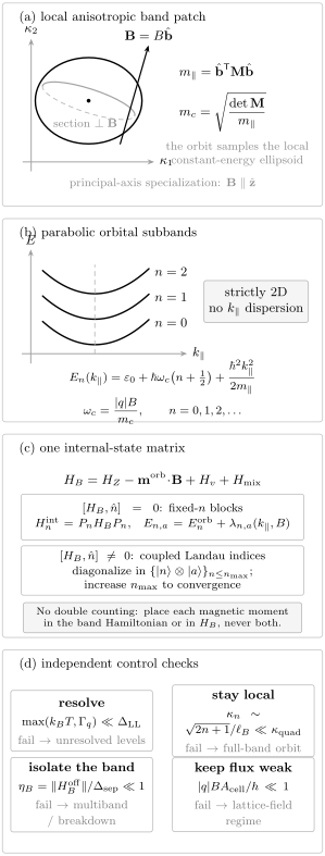
Material Landau-level ledger. A local mass tensor fixes the orbital ladder and longitudinal dispersion. Internal terms may be diagonalized at fixed $n$ only when they preserve Landau index; otherwise the coupled orbital–internal basis must be truncated and convergence checked. Independent model-control and resolution tests delimit the field window in which an observed branch can be assigned. The vertically stacked ledger keeps every panel legible on narrow viewports while preserving the same reading order on larger screens.

Worked Example: Six Silicon Valleys at 10 T

Treat bulk silicon’s six conduction valleys as ideal ellipsoids with representative low-temperature cyclotron-resonance masses reported by Dresselhaus, Kip, and Kittel,

$$m_l=0.916m_e, \qquad m_t=0.190m_e,$$

where $m_l$ is along a valley axis and $m_t$ is transverse. Take $\mathbf B=10\,\mathrm T\,\hat{\mathbf z}$, ignore strain and intervalley coupling, and use a scalar $g^*=2.00$ only for an illustrative spin estimate.

For the two $\pm z$ valleys, the field lies along the longitudinal axis, so

$$m_c^{(\pm z)}=m_t=0.190m_e, \qquad m_{\parallel}^{(\pm z)}=m_l=0.916m_e.$$

For the four $\pm x,\pm y$ valleys, the transverse orbit samples one longitudinal and one transverse mass:

$$m_c^{(\perp z)} = \sqrt{m_lm_t} = 0.417m_e, \qquad m_{\parallel}^{(\perp z)}=m_t=0.190m_e.$$

Using $\hbar e/m_e=0.1158\,\mathrm{meV/T}$ gives

$$\begin{aligned} \hbar\omega_c^{(\pm z)} &= \frac{1.158\,\mathrm{meV}}{0.190} = 6.09\,\mathrm{meV}, \\ \hbar\omega_c^{(\perp z)} &= \frac{1.158\,\mathrm{meV}}{0.417} = 2.78\,\mathrm{meV}. \end{aligned}$$

Thus the orbital zero-point terms differ by

$$\frac12 \left( 6.09-2.78 \right)\,\mathrm{meV} = 1.66\,\mathrm{meV}.$$

The field therefore reorganizes the valley energies even before an explicit valley moment is added: two valleys and four valleys acquire different orbital ladders. This is an orbital-mass effect, not automatically an intrinsic zero-field valley splitting.

Three checks keep the number meaningful. First, $\ell_B=25.66\,\mathrm{nm}/\sqrt{10}=8.12\,\mathrm{nm}$, much larger than the approximately $0.543\,\mathrm{nm}$ silicon lattice parameter certified in NIST SRM 640d. Second, using the conventional cubic-cell face $a^2$ as a representative microscopic area scale gives $Ba^2/(h/e)\simeq7.1\times10^{-4}$, so the lattice-flux test is favorable; this is not a claim that $a^2$ is a primitive-cell area. Third, at $T=4\,\mathrm K$, $k_{\mathrm B}T\simeq0.345\,\mathrm{meV}$; if the Lorentzian quantum half width were $\Gamma_q=0.50\,\mathrm{meV}$, both orbital spacings would be resolvable by the energy-scale test.

The illustrative spin splitting is

$$|g^*|\mu_BB = 2(0.05788\,\mathrm{meV/T})(10\,\mathrm T) = 1.16\,\mathrm{meV}.$$

It exceeds the assumed thermal and disorder scales but is smaller than either orbital spacing. This conclusion is conditional: an interface, confinement, strain, many-body enhancement, or a fitted total $g$ tensor changes the internal ledger and must be declared before comparison with data. The example also does not supply $E_{\mathrm{np}}$, $\kappa_{\mathrm{quad}}$, interband matrix elements, a breakdown field, or a dielectric-screening model from which to audit $E_C$. It therefore demonstrates selected numerical scale checks rather than certifying the complete field window or a one-particle interpretation.

From a Ladder to Oscillations or Hall Physics

A list of eigenvalues is not yet an experimental inference. Quantum Oscillations owns inverse-field periodicity, Lifshitz–Kosevich amplitudes, Dingle analysis, phase conventions, background subtraction, and assignment uncertainty. A measured frequency primarily constrains an extremal orbit area; a temperature-dependent amplitude constrains an orbit cyclotron mass. Neither observation alone identifies a valley, carrier sign, or microscopic band model.

A Landau ladder is also not yet a quantum Hall phase. Integer Quantum Hall Effect owns filling, localization, chiral edges, Hall plateaus, and the link between topology and a measured resistance. Interactions can further reorganize partially filled levels into physics that no single-particle mass tensor predicts. This page stops once the controlled material Hamiltonian and its one-particle spectrum have been identified.

Between weak-field trajectories and resolved levels there is no universal sharp boundary. Semiclassical Dynamics of Bloch Electrons owns the packet equations and their breakdown tests. The same material can support semiclassical motion for a broad distribution while showing quantum oscillations from the coherent subset near the chemical potential.

Reporting a Material Landau Spectrum

A reproducible claim should state:

1. the band source—empirical, $k\cdot p$, tight binding, first-principles, or quasiparticle—and its fitting window;
2. the charge convention, field magnitude and direction, gauge-independent observables, and whether the carrier is an electron or a hole;
3. the full mass tensor or multiband Hamiltonian, not only one scalar mass;
4. every spin, orbital, valley, layer, and confinement term, with the basis and degeneracies before and after diagonalization;
5. the nonparabolicity, separation, lattice-flux, magnetic-breakdown, and field-texture checks that bound model control;
6. temperature, quantum linewidth, chemical potential, and detector channel that bound visibility; and
7. which conclusions are calculated eigenvalues, fitted parameters, or measured assignments.

This ledger makes comparisons auditable. Quoting only “Landau levels were observed” hides the model, resolution, and ownership boundaries needed to assess the claim.

Common Mistakes

Using the bare mass by reflex. The canonical free-particle ladder contains $m_e$, but a local material band contains the direction-dependent cyclotron mass $m_c$. The Bohr magneton still contains $m_e$, so orbital and Zeeman scales need not share the same effective mass.

Reading the field-parallel mass as the cyclotron mass. For a diagonal ellipsoid and field along axis 3, $m_c=\sqrt{m_1m_2}$ while $m_{\parallel}=m_3$. A tilted field requires the full tensor formula.

Multiplying degeneracies after diagonalization. A nominal factor of two for spin or valleys is valid only if the relevant terms leave that sector unresolved. Count eigenvalues of the declared internal Hamiltonian, then apply only surviving symmetry multiplicities.

Adding an orbital moment to a fitted effective g factor. Remote-band coupling can contribute to both. Without a parameter-level decomposition, adding the terms may count the same physics twice.

Equating resolution with model validity. A spacing larger than $k_{\mathrm B}T$ and $\Gamma_q$ says that levels may be visible. It does not show that a quadratic one-band Hamiltonian remains controlled at that energy or field.

Treating a ladder as a transport or topological result. Eigenvalues do not supply scattering, occupations, localization, contacts, or a Chern response. Oscillation, transport, and Hall claims require the corresponding specialist treatments.

Exercises

1. Principal-axis ellipsoid

An electron valley has principal masses $(m_x,m_y,m_z)$ and $\mathbf B=B\hat{\mathbf z}$. Derive $m_c$ and the three-dimensional spectrum without re-solving the coordinate-space oscillator.

Solution

The transverse inverse-mass block is $\mathsf A=\operatorname{diag}(1/m_x,1/m_y)$ and the off-diagonal block vanishes. Therefore

$$m_c = \frac{1}{\sqrt{\det\mathsf A}} = \sqrt{m_xm_y}, \qquad m_{\parallel}=m_z.$$

Importing the canonical orbital result gives

$$E_{n,k_z} = \varepsilon_0 + \hbar\frac{|q|B}{\sqrt{m_xm_y}} \left(n+\frac12\right) + \frac{\hbar^2k_z^2}{2m_z}.$$

2. Tilted-field cyclotron mass

For the same ellipsoid, show that a field along the unit vector $\hat{\mathbf b}$ has

$$m_c = \sqrt{ \frac{m_xm_ym_z} {m_xb_x^2+m_yb_y^2+m_zb_z^2} }.$$

Solution

For $\mathsf M=\operatorname{diag}(m_x,m_y,m_z)$, one has $\det\mathsf M=m_xm_ym_z$ and

$$\hat{\mathbf b}^{\mathsf T} \mathsf M \hat{\mathbf b} = m_xb_x^2+m_yb_y^2+m_zb_z^2.$$

Substitution into the coordinate-free tensor formula gives the result. It reduces to $\sqrt{m_xm_y}$ when $\hat{\mathbf b}=\hat{\mathbf z}$, providing a principal-axis check.

3. Hole convention

Near a valence maximum let the electron energy be $\varepsilon_e(\boldsymbol\kappa)=\varepsilon_v-\hbar^2\kappa^2/(2m_h)$ with $m_h>0$. Explain why inserting the negative electron curvature directly into $\omega_c=|q|B/m$ is wrong, and write the hole ladder.

Solution

The negative curvature describes how occupied electron energies fall away from the maximum; it is not a positive excitation Hamiltonian. Removing an electron creates a hole with excitation energy

$$\varepsilon_h(\boldsymbol\kappa) = \varepsilon_v-\varepsilon_e(\boldsymbol\kappa) = \frac{\hbar^2\kappa^2}{2m_h}$$

and charge $q_h=+e$. Hence

$$E_{h,n} = E_{h,0} + \hbar\frac{eB}{m_h} \left(n+\frac12\right),$$

before spin and orbital shifts. The positive excitation curvature, not a negative oscillator frequency, is quantized.

4. Spin coincidence

For a scalar parabolic band, find the condition under which the Zeeman splitting equals one orbital spacing. Evaluate the required $g^*$ when $m_c=0.20m_e$.

Solution

Set $|g^*|\mu_BB=\hbar eB/m_c$. Since $\mu_B=e\hbar/(2m_e)$,

$$|g^*| = \frac{2m_e}{m_c}.$$

For $m_c=0.20m_e$, the coincidence occurs at $|g^*|=10$. The field cancels in this ideal linear-in-$B$ comparison. Level broadening and nonlinearity determine whether the crossing is actually resolved.

5. Nonparabolic spacing

In the scalar Kane model at $k_{\parallel}=0$, expand $E_n$ through first order in $\alpha_KX_n$ and show how adjacent spacings change with $n$.

Solution

Using $\sqrt{1+4\alpha_KX}=1+2\alpha_KX-2\alpha_K^2X^2+\cdots$ gives

$$E_n = X_n-\alpha_KX_n^2+O(\alpha_K^2X_n^3), \qquad X_n = \hbar\omega_{c0} \left(n+\frac12\right).$$

Therefore

$$E_{n+1}-E_n = \hbar\omega_{c0} - 2\alpha_K (n+1) (\hbar\omega_{c0})^2 + O(\alpha_K^2).$$

For $\alpha_K>0$, the ladder compresses with increasing $n$.

6. Control versus resolution

At $B=12\,\mathrm T$, a band has $m_c=0.25m_e$, $E_{\mathrm{np}}=18\,\mathrm{meV}$, $\Delta_{\mathrm{sep}}=40\,\mathrm{meV}$, $T=8\,\mathrm K$, and $\Gamma_q=1.2\,\mathrm{meV}$. Audit the lowest three orbital levels $n=0,1,2$ using the page’s energy-scale tests.

Solution

The spacing is

$$\hbar\omega_c = \frac{0.1158\,\mathrm{meV/T}\times12\,\mathrm T}{0.25} = 5.56\,\mathrm{meV}.$$

Also $k_{\mathrm B}T\simeq0.689\,\mathrm{meV}$, so the nearest spacing $\Delta_{\mathrm{LL}}=\hbar\omega_c$ exceeds $\max(k_{\mathrm B}T,\Gamma_q)$ and adjacent levels may be resolved. Their orbital energies are $2.78$, $8.34$, and $13.9\,\mathrm{meV}$ above the edge. All are below $E_{\mathrm{np}}$ and $\Delta_{\mathrm{sep}}$, but $n=2$ is not parametrically below $18\,\mathrm{meV}$. Resolution passes more convincingly than quadratic-band control; the highest level needs a nonparabolicity check rather than an unqualified parabolic fit.

Band isolation cannot be certified from $\Delta_{\mathrm{sep}}$ alone because the problem supplies no off-diagonal field-induced mixing matrix elements. It also supplies neither a microscopic cell area nor a magnetic-breakdown scale $B_0$, so lattice-flux and orbit-integrity tests remain unaudited.

7. Six-valley counting

In the silicon example, suppose strain raises the four $\pm x,\pm y$ valleys by $4.0\,\mathrm{meV}$ at zero field. At $10\,\mathrm T$, compare the spin-averaged $n=0$ energies of those valleys with the $\pm z$ pair. Ignore all other shifts.

Solution

Relative to the unstrained $\pm z$ band edge,

$$E_0^{(\pm z)} = \frac12(6.09\,\mathrm{meV}) = 3.05\,\mathrm{meV},$$

whereas

$$E_0^{(\perp z)} = 4.0\,\mathrm{meV} + \frac12(2.78\,\mathrm{meV}) = 5.39\,\mathrm{meV}.$$

The four-valley set remains $2.34\,\mathrm{meV}$ higher. Its degeneracy is four only if strain and the field introduce no further splitting or mixing within that set.

8. Dirac dimensional check

Verify the dimensions of $v\sqrt{2n\hbar|q|B}$ and determine how the ratio $E_2/E_1$ differs from an equally spaced parabolic ladder measured from its band edge.

Solution

Because $\ell_B^{-2}=|q|B/\hbar$, one may write

$$v\sqrt{2n\hbar|q|B} = \frac{\sqrt{2n}\,\hbar v}{\ell_B},$$

which has units of energy. For the positive gapless Dirac branch, $E_2/E_1=\sqrt2$. A parabolic ladder measured from the band edge has $E_n=\hbar\omega_c(n+1/2)$, so $E_2/E_1=(5/2)/(3/2)=5/3$ if levels are numbered $n=1,2$. The differing ratios are a spectrum-level diagnostic, though disorder, Zeeman shifts, and assignment errors must still be excluded.

References

• Ando, T., Fowler, A. B., and Stern, F., “Electronic properties of two-dimensional systems,” Reviews of Modern Physics 54, 437–672 (1982), doi:10.1103/RevModPhys.54.437 — disorder broadening, quantum lifetimes, and magnetotransport in two-dimensional electron systems.
• Ashcroft, N. W., and Mermin, N. D., Solid State Physics, Holt, Rinehart and Winston, 1976 — band dynamics, effective mass, and magnetic quantization.
• Bastard, G., Wave Mechanics Applied to Semiconductor Heterostructures, Les Éditions de Physique, 1988 — envelope functions, interfaces, and semiconductor effective Hamiltonians.
• Black, D. R., Windover, D., Henins, A., Gil, D. L., Filliben, J. J., and Cline, J. P., “Certification of NIST Standard Reference Material 640d,” Powder Diffraction 26, 155–158 (2011), doi:10.1154/1.3591064 — certified silicon lattice parameter and uncertainty.
• Blount, E. I., “Formalisms of band theory,” Solid State Physics 13, 305–373 (1962), doi:10.1016/S0081-1947(08)60459-2 — field-coupled band theory and magnetic response.
• Dresselhaus, G., Kip, A. F., and Kittel, C., “Cyclotron resonance of electrons and holes in silicon and germanium crystals,” Physical Review 98, 368–384 (1955), doi:10.1103/PhysRev.98.368 — anisotropic masses and multivalley cyclotron resonance.
• Goerbig, M. O., “Electronic properties of graphene in a strong magnetic field,” Reviews of Modern Physics 83, 1193–1243 (2011), doi:10.1103/RevModPhys.83.1193 — Dirac Landau levels and graphene.
• Kane, E. O., “Band structure of indium antimonide,” Journal of Physics and Chemistry of Solids 1, 249–261 (1957), doi:10.1016/0022-3697(57)90013-6 — multiband nonparabolic semiconductor structure.
• Kittel, C., Introduction to Solid State Physics, 8th ed., Wiley, 2005 — semiconductor bands, cyclotron resonance, and effective masses.
• Kohn, W., “Theory of Bloch electrons in a magnetic field: the effective Hamiltonian,” Physical Review 115, 1460–1478 (1959), doi:10.1103/PhysRev.115.1460 — effective band Hamiltonians in magnetic fields.
• Luttinger, J. M., “Quantum theory of cyclotron resonance in semiconductors: general theory,” Physical Review 102, 1030–1041 (1956), doi:10.1103/PhysRev.102.1030 — multiband cyclotron resonance.
• McClure, J. W., “Diamagnetism of graphite,” Physical Review 104, 666–671 (1956), doi:10.1103/PhysRev.104.666 — early magnetic quantization of a band-touching system.
• Roth, L. M., “$g$ factor and donor spin-lattice relaxation for electrons in germanium and silicon,” Physical Review 118, 1534–1540 (1960), doi:10.1103/PhysRev.118.1534 — effective Zeeman parameters and remote-band effects.
• Roth, L. M., Lax, B., and Zwerdling, S., “Theory of optical magneto-absorption effects in semiconductors,” Physical Review 114, 90–104 (1959), doi:10.1103/PhysRev.114.90 — interband coupling, orbital terms, and magneto-optics.
• Shoenberg, D., Magnetic Oscillations in Metals, Cambridge University Press, 1984, doi:10.1017/CBO9780511897870 — orbit quantization and quantum-oscillation interpretation.
• Winkler, R., Spin–Orbit Coupling Effects in Two-Dimensional Electron and Hole Systems, Springer, 2003, doi:10.1007/b13586 — matrix effective Hamiltonians, Zeeman terms, and spin–orbit coupling.
• Yu, P. Y., and Cardona, M., Fundamentals of Semiconductors: Physics and Materials Properties, 4th ed., Springer, 2010, doi:10.1007/978-3-642-00710-1 — semiconductor parameters, multivalley bands, and magneto-optical response.