Kondo Effect

The Kondo effect is the many-body screening of a localized magnetic degree of freedom by low-energy electrons in a conducting environment. In the ordinary spin-$1/2$, one-channel case, antiferromagnetic exchange drives a crossover from an approximately free local moment at high temperature to an entangled singlet and a local Fermi liquid at low temperature. The crossover reorganizes scattering, thermodynamics, and spectroscopy around an emergent scale called the Kondo temperature $T_K$.

This page is the canonical home for the material phenomenon and its diagnosis:

• how a magnetic impurity is realized in an alloy, surface system, molecule, or quantum dot;
• why a dilute alloy can have a resistivity minimum;
• what can and cannot be inferred from logarithmic temperature dependence;
• how $T_K$ is defined operationally and tuned experimentally;
• what the screening cloud means as a spatial correlation pattern;
• how single-impurity physics leads into Kondo lattices and heavy-fermion materials.

The Kondo Model Preview owns the exchange-model formalism, perturbative logarithm, one-loop flow, impurity thermodynamics, and low-energy fixed point. The Anderson Impurity Model Preview owns local-moment formation from a fluctuating impurity orbital. Schrieffer–Wolff Transformation owns the controlled elimination of virtual charge states. Heavy Fermions owns the cross-probe diagnosis of the coherent lattice state. Those derivations and lattice consequences are summarized here only far enough to connect them to impurity measurements.

Required background. Kondo Model Preview supplies the exchange model, renormalization-group flow, and fixed-point language.

Helpful background. Exchange Interactions provides the mechanism comparison, Boltzmann Transport provides resistivity language, and the Anderson Impurity Model Preview explains local-moment formation.

Material Ingredients

A Kondo interpretation begins with a ledger of physical ingredients. A low-temperature anomaly is not enough.

A stable local moment

An atom, defect, molecule, or confined electronic level must retain a low-energy spin or pseudospin. For a single correlated orbital with energy $\epsilon_d$, charging energy $U$, and chemical potential $\mu$, the local-moment window is schematically

$$\epsilon_d < \mu < \epsilon_d+U.$$

Hybridization broadens the orbital by an energy $\Gamma$. A recognizable local moment requires charge fluctuations to be sufficiently costly on the scale of $\Gamma$ and temperature. Outside that regime, mixed-valence fluctuations can produce a broad zero-bias feature without a clean separation between charge and spin scales.

In a bulk host, the moment may arise from a transition-metal impurity, a rare-earth ion, an actinide ion, a vacancy, or a correlated cluster. In a quantum dot, an odd-occupancy Coulomb-blockade valley often supplies an effective spin-$1/2$. In scanning-tunnelling experiments, a magnetic adatom or molecule can play the same role.

A bath with low-energy states

The environment must provide electronic states capable of exchanging spin with the moment. For the textbook metallic effect, the local density of states at the Fermi energy is smooth and nonzero:

$$\rho_0 \equiv \rho_{\mathrm{loc}}(E_{\mathrm F}) > 0.$$

Here $\rho_0$ is the local density of states per spin. A gap, pseudogap, superconducting gap, strong spin polarization, or finite-size level spacing can interrupt the flow toward ordinary screening. The bath geometry also determines how many independent screening channels couple to the moment.

Antiferromagnetic exchange

Using the convention

$$H_{\mathrm{int}} = J_K\,\mathbf S\cdot\mathbf s(0),$$

the ordinary Kondo effect requires $J_K>0$. This is antiferromagnetic exchange. Some historical papers define the exchange term with an overall minus sign, so their antiferromagnetic coupling is written with the opposite sign. The Hamiltonian, not the symbol alone, fixes the physics.

Dilution or controlled isolation

The single-impurity picture assumes that moments can be treated independently over the temperature range of interest. In an alloy this requires a sufficiently small impurity concentration. At higher concentrations, indirect exchange, disorder, clustering, and lattice coherence can compete with single-impurity screening. A quantum dot provides a cleaner realization because occupancy, level position, tunnel coupling, field, and bias can often be adjusted independently.

Minimal Low-Energy Description

After impurity charge excitations have been removed, the conventional one-channel Hamiltonian is

$$\begin{aligned} H &= H_c + J_K\,\mathbf S\cdot\mathbf s(0) + W\,n(0), \\ H_c &= \sum_{k,\sigma} \epsilon_k c_{k\sigma}^{\dagger}c_{k\sigma}. \end{aligned}$$

$W$ describes potential scattering. It can alter line shapes and phase shifts, but it does not by itself generate spin screening. The dimensionless bare exchange is

$$g_0 = \rho_0J_K.$$

For $g_0>0$, repeated spin-flip scattering increases the effective coupling as the probe energy is lowered. In the one-loop convention used here,

$$\frac{dg}{d\ell} = 2g^2, \qquad \ell = \ln\frac{D_0}{E}.$$

The solution is

$$g(E) = \frac{g_0} {1-2g_0\ln(D_0/E)}.$$

This formula is controlled only while $g(E)\ll1$. Its apparent pole marks the failure of weak coupling, not a divergent observable. The formal derivation and its density-of-states conventions live in Kondo Model Preview.

The Kondo Temperature

The scale at which the running coupling becomes strong is exponentially smaller than the electronic cutoff:

$$k_{\mathrm B}T_K \sim D_0 \exp\left[ - \frac{1}{2\rho_0J_K} \right].$$

This expression uses a per-spin $\rho_0$ and the one-loop beta function above. If a spin-summed density of states $\rho_{\mathrm{tot}}=2\rho_0$ is used, the same exponent is written $-1/(\rho_{\mathrm{tot}}J_K)$. Higher-order scaling, band shape, potential scattering, and the chosen observable modify the prefactor.

The exponential is physically decisive. Modest changes in hybridization, pressure, local coordination, carrier density, or gate voltage can move $T_K$ by orders of magnitude. It also explains why Kondo correlations may be visible at kelvin scales even when the host bandwidth is measured in electronvolts.

There is no unique numerical definition

$T_K$ labels a universal crossover, but its numerical value depends on the convention used to locate that crossover. Common operational definitions use:

• the zero-temperature impurity susceptibility;
• a specified fraction of the impurity entropy $S_{\mathrm{imp}}(T)$;
• the half-width of a zero-bias spectral feature after deconvolution;
• the half-maximum of a quantum-dot conductance curve;
• a fitted universal scaling function for conductance, susceptibility, or heat capacity;
• a renormalization-group convention tied to the running coupling.

Two careful analyses can therefore report Kondo temperatures differing by a constant factor while describing the same device. A quoted value should name the observable, fit function, and convention.

Gate-controlled Anderson estimate

For a single-level Anderson impurity with $-U<\epsilon_d<0$, a commonly used asymptotic estimate is

$$k_{\mathrm B}T_K \sim \sqrt{\frac{U\Gamma}{2}}\, \exp\left[ \frac{\pi\epsilon_d(\epsilon_d+U)} {2U\Gamma} \right].$$

The prefactor is convention dependent, and the expression is not reliable deep in mixed valence. It nevertheless explains two robust observations: $T_K$ rises rapidly as tunnel coupling grows, and it is usually smallest near the center of an odd-occupancy Coulomb-blockade valley.

Perturbations measured against the scale

Thermal energy, Zeeman energy, and source–drain bias compete with screening through the ratios

$$\frac{T}{T_K}, \qquad \frac{g\mu_{\mathrm B}B}{k_{\mathrm B}T_K}, \qquad \frac{eV}{k_{\mathrm B}T_K}.$$

Universal scaling is expected only after nonuniversal backgrounds, lead asymmetry, voltage division, orbital effects, and heating are controlled. A magnetic field does not generally split a measured zero-bias peak at one universal value of $B/T_K$; instrumental broadening and the observable itself matter.

Why a Resistance Minimum Appears

The historical signature is a minimum in the resistivity of a dilute magnetic alloy. A useful decomposition is

$$\rho(T) = \rho_{\mathrm{res}} + \rho_{\mathrm{ph}}(T) + c_{\mathrm{imp}}\, \Delta\rho_K(T) + \Delta\rho_{\mathrm{other}}(T),$$

where $c_{\mathrm{imp}}$ is the magnetic-impurity concentration. On cooling, the phonon contribution decreases. In the weak-coupling Kondo regime, spin-flip scattering grows, so the two trends can produce a minimum.

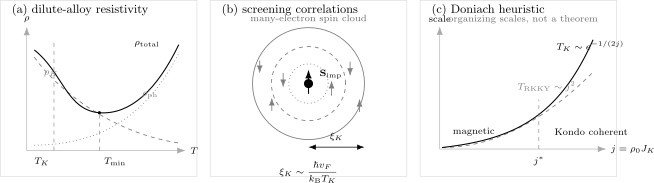
Three distinct uses of the Kondo scale. (a) A phonon background and an increasing magnetic-impurity contribution can produce a minimum at $T_{\min}$; that balance point is not generally $T_K$. (b) The screening length $\xi_K$ characterizes a many-electron spin-correlation pattern rather than a charged orbit. (c) The Doniach comparison of $T_K$ and $T_{\mathrm{RKKY}}$ is a useful organizing heuristic, not a universal phase boundary.

Perturbative logarithm

For $T\gg T_K$, the leading-logarithmic scattering strength behaves schematically as

$$\Delta\rho_K(T) \propto g^2(k_{\mathrm B}T) \sim \frac{1} {4\ln^2(T/T_K)}.$$

Expanding this result at weak bare coupling reproduces the logarithmic increase found in perturbation theory. Neither form should be extrapolated through $T\sim T_K$ into zero temperature.

For a simple low-temperature phonon law and a perturbative logarithm,

$$\rho(T) = \rho_0 + aT^5 + c\ln\frac{T_0}{T},$$

the minimum occurs where

$$T_{\min} = \left( \frac{c}{5a} \right)^{1/5}.$$

If $c$ is proportional to impurity concentration, this gives the classic $c_{\mathrm{imp}}^{1/5}$ scaling. The result is a balance between two temperature derivatives. It does not identify $T_{\min}$ with $T_K$.

Strong-coupling saturation

For a fully screened spin-$1/2$ impurity, scattering approaches the unitary local-Fermi-liquid limit. In an ideal dilute alloy,

$$\Delta\rho_K(T,B) = \rho_u \left[ 1 - c_T \left( \frac{T}{T_K} \right)^2 - c_B \left( \frac{g\mu_{\mathrm B}B} {k_{\mathrm B}T_K} \right)^2 + \cdots \right],$$

with positive coefficients that depend on conventions and geometry. The low-temperature impurity resistivity saturates rather than continuing to grow logarithmically.

In an odd-occupancy quantum dot, the same strong-coupling resonance can instead increase the two-terminal conductance toward a unitary limit:

$$G(T,V,B) = G(0) \left[ 1 - \widetilde c_T \left( \frac{T}{T_K} \right)^2 - \widetilde c_V \left( \frac{eV}{k_{\mathrm B}T_K} \right)^2 - \widetilde c_B \left( \frac{g\mu_{\mathrm B}B} {k_{\mathrm B}T_K} \right)^2 + \cdots \right].$$

The opposite-looking trends are not a contradiction. A bulk resistivity measures impurity-induced backscattering, whereas a dot in series conducts through the interacting level.

A logarithm is not a fingerprint

A resistance upturn approximately linear in $\ln T$ can also arise from weak localization, interaction corrections in disordered conductors, granular transport, structural two-level systems, or a crossover in carrier density. A credible Kondo assignment should seek several mutually consistent signatures:

1. independent evidence for local moments;
2. systematic scaling with magnetic-impurity concentration or dot occupancy;
3. suppression or crossover under a Zeeman field of the expected scale;
4. saturation or Fermi-liquid behavior below the inferred $T_K$;
5. thermodynamic or spectroscopic evidence using the same scale;
6. dimensionality and field dependence inconsistent with the leading localization correction.

Magnetoresistance alone is not decisive because orbital transport, weak localization, spin-disorder scattering, and multiband effects can all respond to field.

Screening and the Kondo Cloud

Above $T_K$, the impurity acts approximately as a free moment with weak, scale-dependent coupling to the bath. Below $T_K$, a spin-$1/2$ impurity coupled to one channel is absorbed into an entangled many-body singlet. “Screening” means that the bath carries compensating spin correlations; it does not mean that one conduction electron occupies a hydrogen-like orbit around the impurity.

A natural spatial observable is

$$C(\mathbf r) = \left\langle \mathbf S_{\mathrm{imp}} \cdot \mathbf s(\mathbf r) \right\rangle.$$

$C(\mathbf r)$ can oscillate on the Fermi-wavelength scale while its envelope crosses over on the much larger Kondo length

$$\xi_K \sim \frac{\hbar v_F} {k_{\mathrm B}T_K}.$$

The precise spatial profile depends on dimension, band structure, channel geometry, temperature, and which correlator is measured. $\xi_K$ is therefore a crossover length, not a sharp boundary. The cloud carries spin correlations with little or no accompanying long-range charge accumulation.

Why direct detection is difficult

For $v_F\sim10^6\,\mathrm{m\,s^{-1}}$ and $T_K\sim10\,\mathrm K$, $\xi_K$ is of order a micrometre. That is enormous compared with a lattice spacing, yet ordinary bulk probes average over many impurities and over rapid $2k_F$ oscillations. Surface disorder, dephasing, finite temperature, and competing impurities further obscure the envelope.

Mesoscopic devices turn the large length into an advantage. If a coherent reservoir or interferometer arm has size $L$ comparable to $\xi_K$, finite-size changes in conductance or phase can reveal the crossover. Borzenets and collaborators reported such evidence in a quantum-dot interferometer by tuning the effective reservoir size. The result is strong evidence for the predicted scale dependence in a controlled device; it should not be described as a real-space image of a universal bulk cloud.

Thermodynamic Signatures

Transport is only one projection of the crossover.

Entropy

In the local-moment regime of an isolated spin-$1/2$,

$$S_{\mathrm{imp}} \longrightarrow k_{\mathrm B}\ln2.$$

For the fully screened one-channel problem,

$$S_{\mathrm{imp}} \longrightarrow 0 \qquad (T\to0).$$

The missing entropy is not destroyed. It is redistributed through impurity–bath entanglement and released through the crossover contribution to the heat capacity.

Susceptibility and heat capacity

At high temperature, the impurity contribution is approximately Curie-like:

$$\chi_{\mathrm{imp}}(T) \sim \frac{(g\mu_{\mathrm B})^2} {4k_{\mathrm B}T} \qquad (S=1/2).$$

Screening cuts off this divergence, leaving a finite $\chi_{\mathrm{imp}}(0)$ of order $1/T_K$. The low-temperature impurity heat capacity is linear,

$$C_{\mathrm{imp}} \sim \gamma_{\mathrm{imp}}T.$$

For the ideal particle–hole-symmetric spin-$1/2$ Kondo model, the appropriately normalized Wilson ratio approaches $2$. In a real material, subtracting host backgrounds, crystal-field levels, inter-impurity coupling, and nuclear terms can be more uncertain than the universal impurity prediction.

Spectroscopy and Nanostructures

Tunnelling line shapes

Scanning tunnelling spectroscopy near a magnetic adatom often shows an asymmetric low-bias anomaly. Interference between tunnelling into a broad conduction channel and into an impurity-mediated channel motivates the phenomenological Fano form

$$\frac{dI}{dV} = G_{\mathrm{bg}} + A \frac{(q+\varepsilon)^2} {1+\varepsilon^2}, \qquad \varepsilon = \frac{eV-E_0}{\Gamma_K}.$$

$q$ is an interference parameter, and $\Gamma_K$ is a fitted width. The line shape is not the impurity spectral function itself, and $\Gamma_K/k_{\mathrm B}$ is not automatically a convention-independent $T_K$. Temperature scaling, field response, adsorption-site dependence, and microscopic modelling are needed.

Quantum dots

A semiconductor quantum dot offers a tunable impurity:

• Coulomb blockade identifies charge sectors;
• odd occupancy supplies a local spin;
• gate voltage adjusts $\epsilon_d$;
• barrier voltages adjust $\Gamma$;
• source–drain bias probes nonequilibrium response;
• a magnetic field controls Zeeman energy.

The characteristic signature is enhanced zero-bias conductance in an odd valley, followed by scaling with $T/T_K$, $eV/(k_{\mathrm B}T_K)$, and $g\mu_{\mathrm B}B/(k_{\mathrm B}T_K)$. Agreement across those axes is much stronger evidence than a zero-bias peak alone. Cotunnelling thresholds, superconducting coherence peaks, weak localization, heating, and accidental resonances are common alternatives.

From One Impurity to a Kondo Lattice

When a local or nearly local $f$-electron degree of freedom occurs in every primitive cell, the same conduction sea couples to a dense array of moments. The antiferromagnetic exchange and the single-impurity convention for $T_K$ remain useful local inputs, but the many-body problem is no longer a sum of independent screening centers.

The lattice adds conduction-mediated intersite exchange, translational coherence, a Fermi-volume question, and the possibility of ordered or fractionalized phases. Its resistivity maximum need not coincide with the impurity $T_K$, and its low-temperature state cannot be inferred by multiplying a single-impurity response by the number of sites.

Kondo Lattices is the canonical home for the dense Hamiltonian, Kondo–RKKY competition, the Doniach heuristic, heavy-Fermi-liquid formation, Fermi-volume counting, and Kondo-breakdown scenarios. Heavy Fermions owns the corresponding material evidence, effective-mass ledger, coherence diagnostics, and representative compounds.

Boundaries and Variants

The ordinary screened singlet is not the outcome of every exchange-coupled impurity.

Setting	Low-energy issue	Why the basic material diagnosis changes
Ferromagnetic $J_K$	coupling is marginally irrelevant	no conventional strong-coupling screening scale
More impurity spin than channel capacity	underscreening	a residual moment survives
More channels than needed	overscreening	non-Fermi-liquid boundary fixed point may appear
Several orbitals or crystal-field states	multistage or anisotropic screening	more than one crossover scale can occur
Pseudogapped bath	depleted low-energy density of states	screened and local-moment phases can be separated by a critical point
Superconducting bath	gap competes with $T_K$	singlet–doublet competition and subgap states replace metallic scaling
Mixed-valence impurity	charge and spin scales overlap	a Kondo-only Hamiltonian may be too narrow
Dense moment array	RKKY and coherence	single-impurity additivity fails

Two-channel Kondo behavior, charge Kondo effects, orbital Kondo effects, and topological or superconducting hosts each require an explicit identification of the effective pseudospin, bath channels, and symmetry protection.

Experimental Inference Workflow

1. Establish the moment

Identify the relevant charge state, ionic configuration, crystal-field multiplet, Curie contribution, or spin-sensitive spectroscopic signature. State whether the low-energy object is a real spin, orbital pseudospin, charge doublet, or another degeneracy.

2. Establish the bath

Measure or model the local low-energy density of states. Record dimensionality, carrier density, Fermi velocity, gaps, spin polarization, and finite-size level spacing. A metallic bulk formula is not portable to a pseudogap or superconducting host without modification.

3. Build an energy-scale ledger

Compare

$$k_{\mathrm B}T, \quad eV, \quad g\mu_{\mathrm B}B, \quad \Gamma, \quad \Delta, \quad k_{\mathrm B}T_K, \quad k_{\mathrm B}T_{\mathrm{RKKY}},$$

where $\Delta$ may denote a superconducting, crystal-field, or finite-size gap. Name how each scale was extracted.

4. Demand cross-observable consistency

Fit scaling functions only in their controlled regimes. Check whether the $T_K$ inferred from transport is compatible, up to declared convention factors, with susceptibility, heat capacity, resonance width, entropy, or finite-size response.

5. Test alternatives

Vary impurity concentration, gate occupancy, sample size, field orientation, disorder, and contact configuration. A mechanism is credible when it predicts how the anomaly changes under these controls, not merely when it fits one temperature trace.

6. Decide whether the problem is dilute or collective

Look for concentration linearity and independent-impurity scaling. Magnetic ordering, spin-glass freezing, a coherence maximum, a reconstructed Fermi surface, or strong site-to-site coupling signals that a lattice or multi-impurity description is needed.

Common Mistakes

Equating the resistivity minimum with the Kondo temperature

$T_{\min}$ depends on the phonon background and impurity concentration. $T_K$ characterizes the many-body crossover of the impurity coupling. They can differ substantially.

Extending the logarithm to zero temperature

Perturbation theory fails near $T_K$. A fully screened impurity reaches a finite strong-coupling scattering limit with quadratic low-energy corrections.

Calling the cloud one bound electron

The cloud is a collective spin-correlation pattern involving particle–hole excitations near the Fermi surface. Its long length does not imply a comparable charge-density halo.

Reading a Fano peak as a spectral function

The measured tunnelling conductance includes interference matrix elements and instrumental broadening. A Fano fit can be useful without uniquely establishing Kondo physics.

Using one universal numerical Kondo temperature

Susceptibility, entropy, spectral-width, and conductance definitions differ by fixed factors even in the ideal model. Materials add further background and model uncertainty.

Treating a Kondo lattice as independent impurities

RKKY interactions and lattice coherence create collective scales and phases. A broad resistivity maximum in a heavy-fermion compound is not interpreted by the same balance equation as a dilute-alloy minimum.

Treating the Doniach crossing as a theorem

The two scale estimates suppress band structure, frustration, valence fluctuations, disorder, and critical dynamics. They organize possibilities; they do not calculate a material phase boundary.

Exercises

Exercise 1: Exponentially small scale

Use the one-loop convention

$$k_{\mathrm B}T_K = D_0e^{-1/(2g_0)}$$

with $g_0=0.08$ and $D_0=1.0\,\mathrm{eV}$. Estimate $T_K$ in kelvin using $1\,\mathrm{eV}/k_{\mathrm B}=1.1605\times10^4\,\mathrm K$.

Solution

The exponent is

$$- \frac{1}{2g_0} = - \frac{1}{0.16} = -6.25.$$

Therefore

$$k_{\mathrm B}T_K = (1.0\,\mathrm{eV})e^{-6.25} \simeq 1.93\times10^{-3}\,\mathrm{eV}.$$

Converting to kelvin gives

$$T_K \simeq (1.93\times10^{-3}) (1.1605\times10^4)\,\mathrm K \simeq 22.4\,\mathrm K.$$

The result is only a one-loop scale in a declared convention. Changing $g_0$ from $0.08$ to $0.10$ would raise the exponential factor from $e^{-6.25}$ to $e^{-5}$, illustrating the strong sensitivity to microscopic parameters.

Exercise 2: Screening length

Estimate

$$\xi_K = \frac{\hbar v_F} {k_{\mathrm B}T_K}$$

for $v_F=1.0\times10^6\,\mathrm{m\,s^{-1}}$ and $T_K=10\,\mathrm K$.

Solution

Using $\hbar=1.055\times10^{-34}\,\mathrm{J\,s}$ and $k_{\mathrm B}=1.381\times10^{-23}\,\mathrm{J\,K^{-1}}$,

$$\begin{aligned} \xi_K &= \frac{ (1.055\times10^{-34}) (1.0\times10^6) }{ (1.381\times10^{-23}) (10) } \mathrm m \\ &\simeq 7.64\times10^{-7}\,\mathrm m \\ &\simeq 0.76\,\mu\mathrm m. \end{aligned}$$

This is a crossover length for spin correlations. It is not the radius of a localized charge orbital.

Exercise 3: Position of a resistance minimum

Suppose

$$\rho(T) = \rho_0 + aT^5 + c\ln\frac{T_0}{T}, \qquad a,c>0.$$

Find $T_{\min}$. If $c$ is proportional to impurity concentration $x$, how does $T_{\min}$ scale with $x$?

Solution

Differentiate:

$$\frac{d\rho}{dT} = 5aT^4 - \frac{c}{T}.$$

At the minimum,

$$5aT_{\min}^5 = c,$$

so

$$T_{\min} = \left( \frac{c}{5a} \right)^{1/5}.$$

If $c\propto x$, then $T_{\min}\propto x^{1/5}$. This concentration dependence belongs to the balance between the phonon and impurity slopes. The intrinsic single-impurity $T_K$ need not have that dependence in a dilute series.

Exercise 4: Same fixed point, opposite transport trends

Why does Kondo screening increase the low-temperature impurity resistivity of a dilute alloy but often increase the low-temperature conductance through an odd-occupancy quantum dot?

Solution

In the alloy, current already flows through the host. The impurity creates an additional scattering channel, and the screened strong-coupling state approaches a large elastic phase shift. Its contribution to bulk resistivity therefore grows and saturates.

In a series quantum dot, current must pass through the interacting level. The Kondo resonance supplies a coherent transmission channel at the Fermi energy. For symmetric coupling and favorable occupancy, the conductance rises toward the unitary limit. The fixed-point phase shift is common to both settings, but the measurement geometries convert it into different transport observables.

Exercise 5: Two Kondo-temperature conventions

One group defines $T_K^{(G)}$ by the half-maximum of a conductance curve. Another defines $T_K^{(\chi)}$ from the zero-temperature impurity susceptibility. Their reported values differ by a factor $1.5$, but both data sets collapse onto the correct universal function after using their own scales. Is one result necessarily wrong?

Solution

No. A crossover has no singular point that fixes one numerical temperature. Different observables and normalization conventions select different constant multiples of the same emergent energy scale.

The comparison becomes meaningful only after each group states its definition and the conversion factor appropriate to the model used. A contradiction would arise if no constant rescaling reconciled the universal curves, or if independently inferred field, bias, and thermodynamic scales were inconsistent beyond experimental and model uncertainty.

Exercise 6: When does the impurity description fail?

A dense intermetallic shows single-impurity scaling above $30\,\mathrm K$, a broad resistivity maximum near $12\,\mathrm K$, and an antiferromagnetic Bragg peak below $4\,\mathrm K$. Which observations require lattice physics, and what ingredients must a low-energy model add beyond one screened impurity?

Solution

The high-temperature collapse can be consistent with predominantly local Kondo scattering. The broad maximum requires care: in a dense material it may mark the onset of lattice coherence or a crossover involving crystal-field levels, so it cannot simply be relabeled $T_K$. The Bragg peak is direct evidence of collective finite-wavevector order and cannot arise from independent impurities.

A minimal lattice description must specify the moment density and lattice, the conduction dispersion and filling, the local exchange $J_K$, and the intersite interaction or susceptibility kernel $I(\mathbf q)$. Crystal-field levels, disorder, and orbital-dependent hybridization may also be necessary. The three temperatures are distinct operational scales until cross-observable evidence shows otherwise.

Exercise 7: Diagnose an incomplete claim

A disordered two-dimensional film has $\rho(T)=\rho_0+A\ln(T_0/T)$ over one decade. The authors call this definitive evidence for Kondo scattering, but report neither moment measurements nor concentration, field, or low-temperature saturation studies. What is missing?

Solution

The logarithm establishes a temperature dependence, not its microscopic origin. In a disordered two-dimensional conductor, weak localization and electron–electron interaction corrections are immediate alternatives.

A stronger study would:

1. establish local moments independently;
2. vary the magnetic-impurity concentration or a controllable charge state;
3. measure field magnitude and orientation dependence;
4. test the expected $T/T_K$ and $g\mu_{\mathrm B}B/(k_{\mathrm B}T_K)$ scaling;
5. extend to low enough temperature to observe saturation or the appropriate fixed-point behavior;
6. compare conductivity corrections with the dimensionality-dependent localization theory;
7. seek a compatible scale in susceptibility, spectroscopy, or another observable.

Until such checks are made, “consistent with Kondo scattering” is defensible; “definitive evidence” is not.

Connections

• Quantum Dots owns confinement, charging, Coulomb diamonds, shell filling, and the device-level route into the odd-occupancy Kondo regime.
• Kondo Model Preview derives the exchange-model flow, thermodynamics, screening cloud, and local Fermi liquid.
• Kondo Model gives the compact model dossier, convention table, methods, and finite-size benchmark.
• Anderson Impurity Model Preview explains local-moment and mixed-valence regimes before charge excitations are removed.
• Anderson Impurity Model provides the compact orbital-model specification and observable–method map.
• Schrieffer–Wolff Transformation derives the low-energy exchange generated by virtual charge fluctuations.
• Exchange Interactions compares direct, superexchange, double-exchange, and conduction-mediated mechanisms.
• RKKY Interaction gives the sign-complete conduction-mediated pair interaction and its Fermi-surface, disorder, and ordering consequences.
• Kondo Lattices owns the dense model, Kondo–RKKY competition, coherence, Fermi-volume counting, and Kondo-breakdown phase vocabulary.
• Heavy Fermions develops the materials evidence for coherent heavy bands, large effective masses, Fermi-volume changes, criticality, and superconductivity.
• Boltzmann Transport provides the semiclassical collision framework whose scale-independent relaxation-time approximation fails for Kondo scattering.
• Drude Theory defines the baseline transport model and the limits of a single phenomenological lifetime.
• Itinerant Magnetism treats collective magnetism of band electrons rather than screening of a distinct local moment.
• Antiferromagnetism develops ordered local-moment and itinerant antiferromagnets reached on the magnetic side of some Kondo lattices.
• Fermi-Liquid Theory Preview gives the bulk quasiparticle framework related to the screened impurity’s local Fermi liquid.
• Quantum Phase Transitions supplies the scaling language needed near field-, pressure-, or composition-tuned zero-temperature transitions.
• Quantum Criticality owns the material endpoint, crossover, thermodynamic, and transport tests beyond the impurity limit.
• Condensed-Matter Roadmap places Kondo phenomenology after bands, transport, exchange, and impurity models.

References

1. P. W. Anderson, “Localized Magnetic States in Metals,” Physical Review 124, 41–53 (1961), doi:10.1103/PhysRev.124.41.
2. J. Kondo, “Resistance Minimum in Dilute Magnetic Alloys,” Progress of Theoretical Physics 32, 37–49 (1964), doi:10.1143/PTP.32.37.
3. J. R. Schrieffer and P. A. Wolff, “Relation between the Anderson and Kondo Hamiltonians,” Physical Review 149, 491–492 (1966), doi:10.1103/PhysRev.149.491.
4. P. W. Anderson, “A Poor Man’s Derivation of Scaling Laws for the Kondo Problem,” Journal of Physics C 3, 2436–2441 (1970), doi:10.1088/0022-3719/3/12/008.
5. K. G. Wilson, “The Renormalization Group: Critical Phenomena and the Kondo Problem,” Reviews of Modern Physics 47, 773–840 (1975), doi:10.1103/RevModPhys.47.773.
6. P. Nozières, “A Fermi-Liquid Description of the Kondo Problem at Low Temperatures,” Journal of Low Temperature Physics 17, 31–42 (1974), doi:10.1007/BF00654541.
7. G. Grüner and A. Zawadowski, “Magnetic Impurities in Non-Magnetic Metals,” Reports on Progress in Physics 37, 1497–1583 (1974), doi:10.1088/0034-4885/37/12/001.
8. A. C. Hewson, The Kondo Problem to Heavy Fermions (Cambridge University Press, 1993), doi:10.1017/CBO9780511470752.
9. E. S. Sørensen and I. Affleck, “Scaling Theory of the Kondo Screening Cloud,” Physical Review B 53, 9153–9167 (1996), doi:10.1103/PhysRevB.53.9153.
10. V. Barzykin and I. Affleck, “The Kondo Screening Cloud: What Can We Learn from Perturbation Theory?,” Physical Review Letters 76, 4959–4962 (1996), doi:10.1103/PhysRevLett.76.4959.
11. I. V. Borzenets et al., “Observation of the Kondo Screening Cloud,” Nature 579, 210–213 (2020), doi:10.1038/s41586-020-2058-6.
12. D. Goldhaber-Gordon et al., “Kondo Effect in a Single-Electron Transistor,” Nature 391, 156–159 (1998), doi:10.1038/34373.
13. S. M. Cronenwett, T. H. Oosterkamp, and L. P. Kouwenhoven, “A Tunable Kondo Effect in Quantum Dots,” Science 281, 540–544 (1998), doi:10.1126/science.281.5376.540.
14. W. G. van der Wiel et al., “The Kondo Effect in the Unitary Limit,” Science 289, 2105–2108 (2000), doi:10.1126/science.289.5487.2105.
15. S. Doniach, “The Kondo Lattice and Weak Antiferromagnetism,” Physica B+C 91, 231–234 (1977), doi:10.1016/0378-4363(77)90190-5.
16. G. R. Stewart, “Heavy-Fermion Systems,” Reviews of Modern Physics 56, 755–787 (1984), doi:10.1103/RevModPhys.56.755.
17. P. Gegenwart, Q. Si, and F. Steglich, “Quantum Criticality in Heavy-Fermion Metals,” Nature Physics 4, 186–197 (2008), doi:10.1038/nphys892.
18. S. Paschen et al., “Hall-Effect Evolution across a Heavy-Fermion Quantum Critical Point,” Nature 432, 881–885 (2004), doi:10.1038/nature03129.