Itinerant Magnetism

Itinerant magnetism is magnetic order or strong magnetic response formed by electrons whose charge and spin remain organized into extended Bloch states or metallic quasiparticles. The electrons that carry the magnetization also participate in the Fermi surface. Magnetic polarization therefore changes band occupations, reconstructs quasiparticle states, and couples collective spin motion to electron–hole excitations.

This definition does not mean that an itinerant magnet has no local moment on any time or length scale. A correlated metal can show atomic Hund physics at short times, a sizable fluctuating moment above its ordering temperature, and a coherent spin-polarized Fermi surface at low temperature. “Localized” and “itinerant” identify useful limiting descriptions; many important materials interpolate between them.

This page owns itinerant magnetism as a material phenomenon:

• spin polarization and exchange splitting of bands;
• uniform and finite-wavevector magnetic instabilities;
• Fermi-surface reconstruction by spin-density-wave order;
• collective transverse modes and the Stoner continuum;
• experimental tests that distinguish a rigid-spin model from an interacting-band description;
• the role of spin fluctuations beyond static mean field.

Stoner Criterion owns the scalar energy-curvature and susceptibility derivations. Fermi-Liquid Theory Preview owns the general quasiparticle energy functional and Landau-parameter response. Random Phase Approximation owns the general bubble-chain resummation, sign conventions, and collective-pole diagnostics. Ferromagnetism and Antiferromagnetism own the corresponding ordered phases whether their microscopic limit is local or itinerant.

Required background. Band Theory Overview supplies bands, occupations, and velocities, while Susceptibilities supplies the source-response and finite-wavevector instability logic.

Helpful background. Fermi Surface and Density of States support state counting; Ferromagnetism and Antiferromagnetism own the resulting ordered phases.

The Magnetic Variable Is a Spin Density

For spin-$1/2$ electron fields, define the dimensionless spin density

$$\hat{\mathbf s}(\mathbf r) = \frac12 \hat\psi^\dagger_\alpha(\mathbf r) \boldsymbol\sigma_{\alpha\beta} \hat\psi_\beta(\mathbf r).$$

Its Fourier components are

$$\hat{\mathbf s}_{\mathbf q} = \int d^3r\, e^{-i\mathbf q\cdot\mathbf r} \hat{\mathbf s}(\mathbf r).$$

A uniform ferromagnet has

$$\left\langle \hat{\mathbf s}_{\mathbf 0} \right\rangle \ne \mathbf 0,$$

whereas an itinerant spin-density wave has

$$\left\langle \hat{\mathbf s}_{\mathbf Q} \right\rangle \ne \mathbf 0$$

at a nonzero ordering wavevector $\mathbf Q$.

The magnetic moment density is related to spin and orbital angular momentum through material-dependent $g$ tensors and spin–orbit coupling in the solid. Even in a nominally spin-only model, sign conventions require care because the electron’s magnetic moment is antiparallel to its spin. It is often cleaner to quote the spin polarization

$$\delta n = n_\uparrow-n_\downarrow$$

and state separately how it is converted to magnetization.

Unlike a rigid-spin model, the magnitude of the itinerant spin density is dynamical. Longitudinal fluctuations can change $\lvert\mathbf s\rvert$ by moving occupation between spin-resolved bands. Transverse fluctuations rotate the polarization and can become collective spin waves. This amplitude freedom is one reason a fixed-$S$ Hamiltonian may fail even when the ordered structure looks simple.

Exchange-Split Bands

A minimal collinear ledger

In a collinear mean-field description without spin–orbit mixing, write

$$\begin{aligned} \varepsilon_{n\mathbf k\uparrow} &= \varepsilon_{n\mathbf k} - \frac12\Delta_{n\mathbf k}, \\ \varepsilon_{n\mathbf k\downarrow} &= \varepsilon_{n\mathbf k} + \frac12\Delta_{n\mathbf k}. \end{aligned}$$

The labels $\uparrow$ and $\downarrow$ refer to a stated quantization axis. The exchange splitting $\Delta_{n\mathbf k}$ need not be constant across bands or momentum. In a multiorbital solid it is generally a matrix in orbital space and can mix with crystal-field and spin–orbit terms.

The spin polarization follows from the occupied states:

$$\delta n = \frac{1}{V} \sum_{n\mathbf k} \left[ f( \varepsilon_{n\mathbf k\uparrow} ) - f( \varepsilon_{n\mathbf k\downarrow} ) \right].$$

At fixed total electron number, exchange splitting also shifts the chemical potential. One cannot generally obtain the magnetic moment by splitting a density-of-states plot while leaving the Fermi level fixed.

Exchange splitting is not a Zeeman field

An externally applied Zeeman field is a controlled source. Exchange splitting is a self-consistent internal energy difference generated by interactions and polarization. In a simple scalar convention,

$$\Delta = I\,\delta n,$$

where $I$ is a Stoner interaction parameter. This equation is a mean-field closure, not a universal definition of $I$. Its numerical value depends on whether $\delta n$ is quoted per atom, per cell, or per volume and on whether the density of states is per spin or spin summed.

Exchange splitting can be large even when the ordered moment is modest if broad regions of momentum contribute with cancellations or if several orbitals polarize differently. Conversely, a spin-resolved photoemission splitting is not by itself proof of a bulk equilibrium ferromagnet; surface magnetism, domains, final-state effects, and matrix elements must be controlled.

Fermi volumes carry the polarization

For a single isotropic three-dimensional band at zero temperature,

$$n_\sigma = \frac{k_{F\sigma}^3}{6\pi^2}.$$

Hence

$$\delta n = \frac{ k_{F\uparrow}^3-k_{F\downarrow}^3 }{6\pi^2}.$$

This simple relation makes the itinerant character concrete: the magnetic polarization is encoded in unequal spin-resolved Fermi volumes. In a real crystal, several sheets, spin–orbit entanglement, and nontrivial band degeneracies replace this scalar picture, but quantum oscillations, angle-resolved photoemission, and first-principles calculations can still test the reconstructed Fermi surface.

Susceptibility as the Organizing Object

Couple a source field to the spin density through

$$\hat H_{\mathrm{src}} = - \sum_{\mathbf q} \mathbf h_{\mathbf q} \cdot \hat{\mathbf s}_{-\mathbf q}.$$

The retarded susceptibility is

$$\chi^{ab}(\mathbf q,\omega) = - \frac{i}{\hbar} \int_0^\infty dt\, e^{i(\omega+i0^+)t} \left\langle \left[ \hat s_{\mathbf q}^a(t), \hat s_{-\mathbf q}^b(0) \right] \right\rangle.$$

It answers three distinct questions:

1. At which wavevector is the paramagnet most susceptible?
2. Does an interaction drive a denominator to zero and create order?
3. In the ordered state, where do collective poles remain sharp relative to the electron–hole continuum?

Independent-particle kernel

For Bloch bands, the bare susceptibility has the schematic form

$$\begin{aligned} \chi_0^{ab}(\mathbf q,\omega) ={}& \frac{1}{V} \sum_{\mathbf k,n,m} \frac{ f(\varepsilon_{n\mathbf k}) - f(\varepsilon_{m,\mathbf k+\mathbf q}) }{ \hbar\omega + \varepsilon_{n\mathbf k} - \varepsilon_{m,\mathbf k+\mathbf q} + i0^+ } \\ &\times \langle n\mathbf k\vert \hat s^a\vert m,\mathbf k+\mathbf q\rangle \langle m,\mathbf k+\mathbf q\vert \hat s^b\vert n\mathbf k\rangle. \end{aligned}$$

The occupation difference supplies phase space, the denominator supplies the electron–hole energy, and the matrix elements encode orbital and spin character. A geometric nesting vector is therefore not sufficient by itself: the relevant states must have nonzero spin matrix elements and an interaction must reinforce that channel.

Interaction enhancement

In a compact matrix Stoner or spin-channel RPA notation,

$$\boldsymbol\chi = \left[ \mathbb 1 - \boldsymbol\chi_0\boldsymbol I \right]^{-1} \boldsymbol\chi_0.$$

The product order and sign follow the source and interaction conventions. A magnetic instability occurs when the largest eigenvalue reaches unity:

$$\lambda_{\max} \left[ \boldsymbol\chi_0(\mathbf q,0) \boldsymbol I \right] = 1.$$

The ordering vector is the $\mathbf q$ at which this happens first. A uniform maximum favors ferromagnetism. A finite-$\mathbf Q$ maximum favors a spin-density wave or itinerant antiferromagnet.

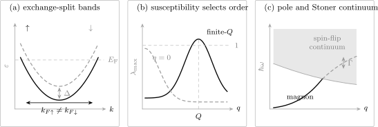
Three linked signatures of itinerant magnetism. Exchange splitting changes the spin-resolved Fermi surfaces; the enhanced susceptibility selects either $\mathbf q=0$ or a finite ordering vector $\mathbf Q$; and a transverse collective mode can remain sharp below the spin-flip electron–hole continuum before broadening when it enters that continuum.

The Scalar Stoner Limit

The dedicated Stoner Criterion page derives this limit and fixes its factor-of-two ledger. For one band, a momentum-independent interaction, and a paramagnetic density of states per spin $N(E_{\mathrm F})$, the uniform static susceptibility takes the mean-field form

$$\chi = \frac{\chi_{\mathrm P}}{ 1-I\,N(E_{\mathrm F}) }.$$

If $N(E_{\mathrm F})$ is per spin and per volume in SI units, the noninteracting Pauli spin susceptibility is

$$\chi_{\mathrm P} = 2\mu_0\mu_B^2 N(E_{\mathrm F}).$$

If the density of states is instead quoted per atom or per cell, $I$ must use the matching normalization. The enhancement factor

$$\mathcal S := \frac{\chi}{\chi_{\mathrm P}} = \frac{1}{ 1-I\,N(E_{\mathrm F}) }$$

diverges at the scalar mean-field threshold

$$I\,N(E_{\mathrm F}) = 1.$$

The criterion captures the competition between the band-energy cost of unequal spin populations and the interaction-energy gain. It is useful because it connects magnetism to the Fermi-level density of states. It is incomplete because it suppresses momentum, orbital structure, self-energy corrections, vertex corrections, and critical spin fluctuations. A large noninteracting density of states is an invitation to test a magnetic instability, not a proof that the ground state is ferromagnetic.

Finite-Wavevector Spin-Density Waves

Define the spin-density-wave order parameter

$$\mathbf m_{\mathbf Q} = \frac{1}{2N} \sum_{\mathbf k} \left\langle c^\dagger_{\mathbf k+\mathbf Q,\alpha} \boldsymbol\sigma_{\alpha\beta} c_{\mathbf k,\beta} \right\rangle.$$

This order coherently mixes quasiparticle states whose momenta differ by $\mathbf Q$. The magnetic unit cell enlarges, the Brillouin zone folds, and avoided crossings open where the original bands intersect their translated copies.

For one coupled sector, the mean-field matrix is

$$\mathcal H_{\mathbf k} = \begin{pmatrix} \varepsilon_{\mathbf k} & \Delta_{\mathbf Q} \\ \Delta_{\mathbf Q}^{*} & \varepsilon_{\mathbf k+\mathbf Q} \end{pmatrix}.$$

The corresponding eigenvalues are

$$\begin{aligned} E_\pm(\mathbf k) ={}& \frac{ \varepsilon_{\mathbf k} + \varepsilon_{\mathbf k+\mathbf Q} }{2} \\ &\pm \sqrt{ \left[ \frac{ \varepsilon_{\mathbf k} - \varepsilon_{\mathbf k+\mathbf Q} }{2} \right]^2 + \lvert\Delta_{\mathbf Q}\rvert^2 }. \end{aligned}$$

Perfect nesting is not required for order, and imperfect nesting does not preclude it. Imperfectly gapped regions can leave reconstructed metallic pockets. Itinerant antiferromagnets are therefore often metals rather than Slater insulators.

Chromium is the classic material example: its incommensurate antiferromagnetism is described by a spin-density wave whose wavevector, Fermi-surface geometry, lattice strain, and accompanying charge modulation are experimentally linked. The example is instructive precisely because a simple nesting cartoon is not the whole material theory; orbital matrix elements, interactions, pressure, alloying, and fluctuations all matter.

Antiferromagnetism owns the ordered-phase classification and the folded-band derivation in its wider local-to-itinerant context.

Collective Modes and the Stoner Continuum

Spin-flip electron–hole excitations

In a collinear spin-polarized metal, a transverse spin operator can remove an occupied majority-spin quasiparticle and create a minority-spin quasiparticle. The allowed continuum contains energies

$$\hbar\omega = \varepsilon_{m,\mathbf k+\mathbf q,\downarrow} - \varepsilon_{n,\mathbf k,\uparrow},$$

subject to

$$f( \varepsilon_{n,\mathbf k,\uparrow} ) = 1, \qquad f( \varepsilon_{m,\mathbf k+\mathbf q,\downarrow} ) = 0$$

at zero temperature. This set of spin-flip electron–hole states is the Stoner continuum.

The continuum is not one sharp dispersion. Its boundaries and spectral weight depend on all pairs of occupied and empty bands connected by $\mathbf q$, including their spin matrix elements.

Collective transverse poles

Broken spin-rotation symmetry requires a low-energy transverse collective mode when spin–orbit coupling and external fields are neglected. In an itinerant ferromagnet, the susceptibility denominator can produce a magnon pole below the Stoner continuum. At small wavevector it can be sharp and quadratic:

$$\hbar\omega_{\mathrm m}(\mathbf q) \simeq Dq^2.$$

As the branch approaches the continuum, it can hybridize with electron–hole states, lose pole residue, and acquire Landau damping. A schematic pole condition is

$$\det \left[ \mathbb 1 - \boldsymbol\chi_0( \mathbf q,\omega ) \boldsymbol I \right] = 0.$$

If $\operatorname{Im}\boldsymbol\chi_0$ is nonzero at the pole, the mode generally has a finite linewidth unless a matrix element or symmetry suppresses the coupling.

Longitudinal fluctuations

Longitudinal response changes the magnitude of the polarization. In a rigid-spin model such amplitude motion is absent by construction. In an itinerant magnet it can be low enough in energy to affect thermodynamics, neutron spectra, and the transition itself. Longitudinal weight often overlaps strongly with particle–hole continua and need not form a sharp amplitude mode.

Spin Waves and Magnons gives the material workflow for comparing collective branches, eigenvectors, cross sections, and linewidths. The canonical Magnons article owns the reusable quantization framework.

Local-Moment and Itinerant Limits

The most useful comparison is operational:

Question	Local-moment limit	Itinerant limit
What carries magnetism?	moments identifiable before long-range order	spin polarization of extended quasiparticle states
What orders?	moment orientation, sometimes multipoles	momentum- and orbital-resolved spin density
Is the amplitude fixed?	approximately, below local excitation scales	generally soft and state dependent
Natural low-energy model	spin Hamiltonian	interacting multiband electron Hamiltonian
Charge sector	may be insulating or metallic	ordinarily metallic
Excitation continuum	multi-spin and fractional channels	spin-flip electron–hole channels
Above the transition	local moment can persist	polarization can weaken, but fluctuating moments can also persist
Parameter language	$S$, exchange tensors, anisotropy	bands, self-energies, vertices, $\chi(\mathbf q,\omega)$

No single measurement places a material permanently in one column.

Scale dependence

A metal can look local on femtosecond time scales and itinerant in its low-energy coherent response. Orbital-selective materials can have some orbitals forming robust moments while others remain mobile. Hund coupling can create a substantial instantaneous moment, while hybridization and intersite coherence determine how that moment orders.

Effective spin models can still work

If transverse collective modes are well separated from longitudinal and electron–hole continua, integrating out the itinerant electrons can produce an effective spin Hamiltonian over a limited energy range. Its exchange couplings may be long ranged, retarded, state dependent, and sensitive to the Fermi surface. Success of a low-energy spin-wave fit does not prove that the microscopic moments were rigid at all energies.

A metal is not automatically itinerant-magnetic

Local moments can coexist with a Fermi surface. Rare-earth metals, Kondo lattices above screening scales, and local-moment metals can conduct through electrons distinct from the moments. The diagnostic question is whether the electrons forming the relevant Fermi surface also form and reshape the magnetic order parameter.

Experimental Diagnostics

Spin-resolved band structure

Spin- and angle-resolved photoemission can resolve exchange-split occupied bands, while inverse photoemission and resonant spectroscopies access unoccupied states. Compare the observed splitting over momentum and orbital character rather than quoting one number.

Quantum oscillations and magnetotransport can reveal spin-split or reconstructed Fermi-surface sheets. Their interpretation requires care with magnetic breakdown, Zeeman splitting, spin–orbit coupling, domains, and field-induced transitions.

Ordered and fluctuating moments

Neutron diffraction measures the spatial Fourier components of the ordered magnetization density. Inelastic neutron scattering measures $\operatorname{Im}\chi(\mathbf q,\omega)$ after form-factor and polarization projection. A sharp low-$q$ magnon that broadens into a continuum is strong itinerant evidence when a band calculation reproduces the continuum kinematics and spectral weight.

X-ray magnetic circular dichroism can separate element-specific spin and orbital contributions subject to sum-rule assumptions. NMR, Mössbauer spectroscopy, and muon spin rotation access local fields and fluctuation time scales. These probes can establish that substantial local magnetism persists above an ordering transition even when the low-temperature phase has an itinerant Fermi surface.

Thermodynamics and the Rhodes–Wohlfarth ratio

Fit the high-temperature susceptibility only over a regime where a Curie–Weiss form is justified:

$$\chi(T) = \chi_0 + \frac{C}{T-\Theta}.$$

The effective moment $p_{\mathrm{eff}}$ is defined through the Curie constant. Rhodes and Wohlfarth introduce $p_c$ by

$$p_{\mathrm{eff}}^2 = p_c(p_c+2)$$

when moments are measured in units of $\mu_B$, and compare it with the low-temperature spontaneous moment $p_s$. A ratio

$$\frac{p_c}{p_s} \gg 1$$

is a classic signature of weak itinerant ferromagnetism: strong fluctuating response coexists with a small ordered moment.

This ratio is a diagnostic, not a binary theorem. Crystal-field moments, orbital contributions, Kondo screening, temperature-dependent backgrounds, unsaturated magnetization, and an inadequate Curie–Weiss window can all distort it.

The electronic heat-capacity coefficient and uniform susceptibility can also be combined into a Wilson ratio. Fermi-Liquid Theory Preview owns its normalization and interpretation. An enhanced Wilson ratio signals strong spin-channel interactions but does not by itself establish ordered itinerant magnetism.

Pressure, composition, and field

Weak itinerant magnets are often sensitive to small changes in lattice spacing, pressure, or composition because those changes reshape the density of states and susceptibility. This sensitivity is informative only with structural and disorder controls. A pressure-driven loss of magnetism can result from bandwidth changes, a first-order transition, competing order, or a change in electronic coherence.

First-Principles and Model Calculations

Spin-polarized density-functional calculations can predict:

• ordered moments and spin density;
• exchange-split band structures;
• magnetic anisotropy with spin–orbit coupling;
• relative energies of candidate magnetic structures;
• momentum-dependent susceptibilities in a chosen approximation.

Agreement with the ordered moment and one band splitting is not enough. A trustworthy comparison also checks Fermi-surface geometry, orbital character, mode energies, transition scales, and sensitivity to the exchange-correlation functional.

Fixed-spin-moment energy

A useful calculation constrains the total moment $M$ and evaluates

$$E_{\mathrm{FSM}}(M).$$

Near $M=0$,

$$E_{\mathrm{FSM}}(M) = E_0 + \frac{a_2}{2}M^2 + \frac{a_4}{4}M^4 + \cdots.$$

A negative $a_2$ signals a uniform mean-field instability in that computational approximation. Multiple minima can indicate metamagnetism or competing magnetic states. The result is still a zero-temperature electronic energy landscape; it does not automatically supply the finite-temperature transition or the fluctuation renormalization.

Dynamic susceptibility

Time-dependent density-functional theory, many-body perturbation theory, dynamical mean-field theory, and model-based RPA calculate different approximations to $\chi(\mathbf q,\omega)$. They differ in self-energy, vertex, locality, and double-counting choices. Comparison should therefore report:

1. the one-particle propagator used;
2. the interaction vertex;
3. whether spin–orbit coupling is retained;
4. the analytic-continuation or broadening procedure;
5. sum-rule and Goldstone checks;
6. the experimental resolution convolution.

Spin Fluctuations Beyond Static Stoner Theory

Static Stoner mean field often predicts the existence and zero-temperature scale of polarization more successfully than it predicts finite-temperature behavior. It neglects the spatial and temporal spin fluctuations that reduce ordered moments, renormalize spectra, and commonly lower calculated transition temperatures.

Moriya’s spin-fluctuation and self-consistent-renormalization framework treats the spectrum of paramagnons as part of the thermodynamics. It explains why itinerant electrons can produce Curie–Weiss-like susceptibility and sizable fluctuating moments without becoming pre-existing rigid spins.

Near a magnetic quantum phase transition, gapless electron–hole excitations cannot always be treated as passive damping. They can alter the effective action of the order parameter and invalidate a purely local Landau expansion. In clean metallic ferromagnets, coupling to soft particle–hole modes can favor a first-order low-temperature transition or modulated phases; a continuous Hertz-type transition is not universal. Material disorder, dimensionality, spin–orbit coupling, and additional phases change the outcome.

Claims of “quantum critical itinerant ferromagnetism” should therefore identify:

• the tuning parameter and phase boundary;
• whether the transition is continuous or first order;
• disorder and residual-resistivity scales;
• the temperature window of any scaling law;
• alternative ordered or inhomogeneous phases;
• whether the measured exponents describe equilibrium criticality or a crossover.

Representative Material Regimes

Iron, cobalt, and nickel

Their spin-polarized Fermi surfaces and band structures establish a major itinerant component. Yet their finite-temperature behavior is not captured uniformly by a bare Stoner model. Iron retains more robust moment amplitude than nickel, while spin fluctuations substantially renormalize transition temperatures and spectra. Treating all three as identical “Stoner ferromagnets” loses the physics.

Chromium

Chromium is the canonical finite-$\mathbf Q$ itinerant antiferromagnet. Its incommensurate spin-density wave, Fermi-surface reconstruction, charge modulation, and pressure or alloy sensitivity make it a benchmark for susceptibility-driven order.

Weak itinerant ferromagnets

Materials such as ZrZn$_2$, Ni$_3$Al, and MnSi have small ordered moments and strong tunability. MnSi additionally has chiral spin–orbit interactions and helimagnetic order, so it is not a scalar Stoner ferromagnet. These systems are valuable precisely because pressure and field expose fluctuation and quantum-transition effects omitted by mean field.

Hund and multiorbital metals

Iron-based superconductors and related multiorbital compounds often show coherent reconstructed bands together with sizable local fluctuating moments. Orbital selectivity, Hund coupling, and nesting all contribute. The local-versus-itinerant question is therefore poorly posed unless an energy, time, orbital, and momentum scale is specified.

Reliable Analysis Workflow

1. Identify the order. Determine the ordering wavevector, moment direction, domains, and thermodynamic transition.
2. Establish metallic degrees of freedom. Map the Fermi surface, carrier density, and orbital character in the relevant phase.
3. Fix conventions. State whether densities of states are per spin and per atom, cell, or volume; state the source sign in $\chi$.
4. Compare uniform and finite-$\mathbf q$ response. Do not apply a scalar Stoner number when the leading susceptibility eigenvalue is at finite wavevector.
5. Test exchange splitting self-consistently. Conserve total charge and compare momentum- and orbital-resolved splittings.
6. Calculate collective and continuum weight. Fit $\operatorname{Re}\chi$ and $\operatorname{Im}\chi$, not only branch energies.
7. Look across scales. Compare ordered, instantaneous, and Curie–Weiss moments rather than forcing them to coincide.
8. Audit fluctuations. Check whether mean field overestimates $T_C$ or $T_N$ and whether paramagnons dominate a measured regime.
9. Use perturbations as tests. Pressure, composition, and field should be modeled together with structural and disorder changes.
10. State the model’s window. An effective spin model, Stoner model, Fermi liquid, or local self-energy theory is never valid at all energies by default.

Common Mistakes

Calling every magnetic metal an itinerant magnet

Local moments can order in a metal while separate conduction electrons carry charge.

Equating small ordered moment with itinerancy

Frustration, Kondo screening, covalency, quantum fluctuations, or noncollinearity can also reduce the measured moment.

Treating exchange splitting as an external Zeeman field

It is a self-consistent interaction effect and changes when occupations, structure, or temperature change.

Using total and per-spin density of states interchangeably

This creates a factor-of-two error in the Pauli susceptibility and Stoner product.

Declaring nesting sufficient

Orbital matrix elements, interaction vertices, self-energy effects, and competing wavevectors must also be tested.

Fitting a sharp magnon without the Stoner continuum

An itinerant collective pole can lose residue and broaden when it overlaps spin-flip electron–hole states.

Treating a DFT moment as an experimental mechanism

A spin-polarized ground state in one functional is evidence for an electronic instability within that approximation, not a complete finite-temperature theory.

Interpreting Curie–Weiss behavior as proof of rigid moments

Collective itinerant spin fluctuations can generate an effective Curie–Weiss regime.

Assuming every metallic quantum ferromagnetic transition is continuous

Soft fermionic modes, disorder, and modulated phases can change or preempt the transition.

Exercises

Exercise 1: Stoner enhancement

A single-band metal has

$$I\,N(E_{\mathrm F}) = 0.80,$$

with $N(E_{\mathrm F})$ defined per spin. Find the scalar Stoner enhancement $\mathcal S=\chi/\chi_{\mathrm P}$. Is the paramagnet unstable in this approximation?

Solution

The enhancement is

$$\mathcal S = \frac{1}{1-0.80} = 5.$$

The susceptibility is strongly enhanced, but the scalar mean-field denominator remains positive. The paramagnet is not yet unstable because $I\,N(E_{\mathrm F})\lt1$.

This conclusion concerns only the uniform scalar channel. A finite-wavevector or multiorbital eigenvalue could still reach unity first.

Exercise 2: Polarization from Fermi volumes

For one isotropic band at zero temperature, let

$$k_{F\uparrow} = 1.05\,\mathrm{nm}^{-1}, \qquad k_{F\downarrow} = 0.95\,\mathrm{nm}^{-1}.$$

Calculate $n_\uparrow-n_\downarrow$.

Solution

Using

$$n_\sigma = \frac{k_{F\sigma}^3}{6\pi^2},$$

gives

$$\begin{aligned} \delta n &= \frac{ (1.05)^3-(0.95)^3 }{6\pi^2} \,\mathrm{nm}^{-3} \\ &= \frac{ 1.157625-0.857375 }{6\pi^2} \,\mathrm{nm}^{-3} \\ &\simeq 5.07\times10^{-3} \,\mathrm{nm}^{-3}. \end{aligned}$$

The corresponding spin-only magnetic-moment magnitude is approximately $\mu_B\delta n$ for $g\simeq2$, subject to the stated spin labeling and electron-moment sign convention.

Exercise 3: Which wavevector orders?

For a multiorbital paramagnet, the largest eigenvalue of

$$\boldsymbol\chi_0(\mathbf q,0) \boldsymbol I$$

is $0.78$ at $\mathbf q=0$ and $1.08$ at an incommensurate $\mathbf Q$. What instability is predicted first by this approximation?

Solution

The finite-$\mathbf Q$ eigenvalue has crossed unity while the uniform eigenvalue has not. The predicted instability is therefore an incommensurate spin-density wave, not a uniform ferromagnet.

The eigenvector of the matrix product identifies the orbital and spin combination that orders. Quoting only a total density of states would miss both the finite wavevector and the multiorbital structure.

Exercise 4: A protected low-energy collective mode

In an ideal isotropic itinerant ferromagnet at zero field, a calculation produces a finite transverse gap at $\mathbf q=0$ even though spin–orbit coupling was omitted. What should be checked?

Solution

Exact spin-rotation symmetry and spontaneous ferromagnetic order require a gapless transverse Goldstone mode. Check:

1. self-consistency of the ordered mean field;
2. consistency between the one-particle self-energy and response vertex;
3. the sign and normalization of the transverse susceptibility;
4. numerical momentum and frequency resolution;
5. whether an explicit field or anisotropy entered inadvertently.

A response approximation that violates the relevant Ward identity can produce a spurious gap even when its ground-state polarization looks reasonable.

Exercise 5: Rhodes–Wohlfarth diagnostic

A ferromagnetic metal has

$$p_{\mathrm{eff}} = 2.83, \qquad p_s = 1.00,$$

in units of $\mu_B$. Compute $p_c$ from

$$p_{\mathrm{eff}}^2 = p_c(p_c+2)$$

and find $p_c/p_s$.

Solution

Solving the quadratic equation gives the positive root

$$p_c = - 1 + \sqrt{ 1+p_{\mathrm{eff}}^2 }.$$

Since $2.83^2\simeq8.01$,

$$p_c \simeq -1+\sqrt{9.01} \simeq 2.00.$$

Therefore

$$\frac{p_c}{p_s} \simeq 2.$$

The ratio larger than one supports an intermediate or itinerant ferromagnetic interpretation, but it is not conclusive without checking the Curie–Weiss window, saturation, orbital moment, and other probes.

Exercise 6: Collective mode entering a continuum

A transverse branch is resolution limited below $30\,\mathrm{meV}$, then broadens rapidly and loses integrated peak weight where a band calculation predicts spin-flip electron–hole states. Give the leading interpretation and two checks.

Solution

The leading interpretation is Landau damping: a collective transverse pole has entered the Stoner continuum and can decay into spin-flip electron–hole excitations.

Two essential checks are:

1. compare the measured onset in both momentum and energy with the matrix-element-weighted continuum, not only its geometric boundary;
2. verify that the missing pole weight is redistributed into magnetic continuum weight after background and resolution corrections.

Additional checks include temperature and polarization dependence, alternative phonon or orbital hybridization, and whether disorder broadening could mimic the onset.

Exercise 7: Local and itinerant evidence together

A metal shows a spin-polarized Fermi surface below $T_C$, a substantial instantaneous moment above $T_C$, and a Curie–Weiss susceptibility over an intermediate temperature range. Must one of these observations be wrong?

Solution

No. The observations probe different scales. Hund and correlation physics can produce a sizable short-time local moment, while low-temperature coherence organizes the same electronic degrees of freedom into spin-polarized quasiparticle bands. Collective spin fluctuations can generate a Curie–Weiss-like regime above the transition.

A successful theory must reproduce the probe time scales, orbital content, ordered moment, Fermi-surface reconstruction, and dynamic susceptibility together. Labeling the material simply “local” or “itinerant” without those qualifiers discards the central evidence.

Connections

• Magnetic Moments in Matter reconciles short-time local, ordered, and thermodynamic moment records and decides when this page’s distributed itinerant description must replace or supplement a fixed-length model.
• Ferromagnetism owns spontaneous uniform order, domains, Curie behavior, and the local-to-itinerant phase comparison.
• Antiferromagnetism owns finite-wavevector magnetic order, magnetic cells, spin flop, and the material spin-density-wave limit.
• Charge and Spin Density Waves compares SDWs with charge order, Peierls mechanisms, reconstruction, collective coordinates, and coexistence tests.
• Fermi Surface and Density of States supply the electronic geometry and counting used by susceptibility and Stoner arguments.
• Fermi-Liquid Theory Preview owns quasiparticle interactions, spin susceptibility, Wilson ratios, and Pomeranchuk stability.
• Random Phase Approximation develops the general response denominator, particle–hole continuum, collective poles, and limitations.
• Susceptibilities fixes source, response, order-of-limits, and unit conventions.
• Spectral Functions owns pole, residue, linewidth, self-energy, and continuum language.
• Spin Waves and Magnons turns magnetic models into probe-weighted spectra and provides linewidth and stability checks.
• Stoner Criterion derives the scalar uniform instability from band-energy curvature, exchange gain, and susceptibility enhancement.
• RKKY Interaction converts the itinerant host susceptibility into exchange between distinct local moments and clarifies the role of Fermi-surface spanning vectors.
• Kondo Effect treats screening of a distinct local moment by itinerant electrons and the heavy-fermion crossover where local-versus-itinerant classification becomes scale dependent.
• Hubbard Model gives a canonical interacting-electron model whose weak- and intermediate-coupling regimes support itinerant magnetic instabilities.
• Hall Effect separates ordinary, anomalous, and quantized transverse responses in magnetic metals.
• Quantum Criticality develops the material tests for field- or pressure-tuned itinerant endpoints, hot-region transport, preemption, and Hertz–Millis boundaries.
• Condensed-Matter Roadmap places itinerant magnetism after band structure, Fermi surfaces, exchange, and magnetic order.

References

1. E. C. Stoner, “Collective Electron Ferromagnetism,” Proceedings of the Royal Society A 165, 372–414 (1938), doi:10.1098/rspa.1938.0066.
2. E. C. Stoner, “Collective Electron Ferromagnetism. II. Energy and Specific Heat,” Proceedings of the Royal Society A 169, 339–371 (1939), doi:10.1098/rspa.1939.0003.
3. P. Rhodes and E. P. Wohlfarth, “The Effective Curie–Weiss Constant of Ferromagnetic Metals and Alloys,” Proceedings of the Royal Society A 273, 247–258 (1963), doi:10.1098/rspa.1963.0086.
4. T. Moriya, Spin Fluctuations in Itinerant Electron Magnetism (Springer, 1985), doi:10.1007/978-3-642-82499-9.
5. J. Kübler, Theory of Itinerant Electron Magnetism, 2nd ed. (Oxford University Press, 2021), doi:10.1093/oso/9780192895639.001.0001.
6. E. Fawcett, “Spin-Density-Wave Antiferromagnetism in Chromium,” Reviews of Modern Physics 60, 209–283 (1988), doi:10.1103/RevModPhys.60.209.
7. L. M. Sandratskii, “Noncollinear Magnetism in Itinerant-Electron Systems: Theory and Applications,” Advances in Physics 47, 91–160 (1998), doi:10.1080/000187398243225.
8. T. Moriya and K. Ueda, “Spin Fluctuations and High Temperature Superconductivity,” Advances in Physics 49, 555–606 (2000), doi:10.1080/000187300412248.
9. H. v. Löhneysen, A. Rosch, M. Vojta, and P. Wölfle, “Fermi-Liquid Instabilities at Magnetic Quantum Phase Transitions,” Reviews of Modern Physics 79, 1015–1075 (2007), doi:10.1103/RevModPhys.79.1015.
10. M. Brando, D. Belitz, F. M. Grosche, and T. R. Kirkpatrick, “Metallic Quantum Ferromagnets,” Reviews of Modern Physics 88, 025006 (2016), doi:10.1103/RevModPhys.88.025006.
11. A. Georges, L. de’ Medici, and J. Mravlje, “Strong Correlations from Hund’s Coupling,” Annual Review of Condensed Matter Physics 4, 137–178 (2013), doi:10.1146/annurev-conmatphys-020911-125045.
12. I. I. Mazin, D. J. Singh, M. D. Johannes, and M. H. Du, “Unconventional Superconductivity with a Sign Reversal in the Order Parameter of LaFeAsO$_{1-x}$F$_x$,” Physical Review Letters 101, 057003 (2008), doi:10.1103/PhysRevLett.101.057003.
13. P. Dai, “Antiferromagnetic Order and Spin Dynamics in Iron-Based Superconductors,” Reviews of Modern Physics 87, 855–896 (2015), doi:10.1103/RevModPhys.87.855.
14. N. W. Ashcroft and N. D. Mermin, Solid State Physics (Holt, Rinehart and Winston, 1976).
15. P. Coleman, Introduction to Many-Body Physics (Cambridge University Press, 2015), doi:10.1017/CBO9781139020916.