Quantum Criticality

Quantum criticality in a material is the finite-temperature and finite-frequency organization produced by a continuous phase transition whose endpoint lies at zero temperature. The endpoint itself is an ideal limit. Experiments infer it from a controlled tuning trajectory, the fate of the adjacent phases, vanishing crossover scales, singular response, and scaling shared by several observables.

That standard is deliberately stronger than observing a resistivity exponent different from two. Linear resistivity, a divergent effective mass, an $E/T$ collapse, or a broad thermodynamic maximum can each occur for more than one reason. A material earns a quantum-critical interpretation when those observations form one consistent phase-diagram and energy-scale ledger.

Canonical Scope

Quantum Phase Transitions owns the general definition of a zero-temperature phase transition, the thermodynamic limit, continuous versus first-order behavior, the quantum-critical fan, and benchmark models. Critical Exponents and Scaling owns the exponent dictionary, homogeneity laws, corrections to scaling, and covariance-aware collapse. Critical Phenomena and RG Bridge owns the continuum-field-theory and renormalization-group bridge.

This page owns material phenomenology and inference:

• how pressure, field, composition, strain, or carrier density tune a candidate endpoint;
• how crossover fans are reconstructed from finite-temperature data;
• which thermodynamic, spectroscopic, and transport signatures constrain the claim;
• how metallic magnetic criticality differs between order-parameter and Kondo-destruction scenarios;
• how disorder, first-order behavior, Fermi-surface topology, and competing phases can imitate or hide criticality;
• which questions remain active rather than settled.

Kondo Lattices owns the dense model and its phase vocabulary. Heavy Fermions owns the materials-facing heavy-band and effective-mass diagnosis. This article uses those results to compare critical scenarios without duplicating their derivations.

From a Control Knob to a Zero-Temperature Endpoint

Let $\lambda$ denote the experimentally controlled variable and define a dimensionless detuning

$$r = \frac{\lambda-\lambda_c}{\lambda_0}.$$

The scale $\lambda_0$ and the sign of $r$ must be stated. A magnetic field in tesla, pressure in gigapascals, and substitution fraction are not interchangeable scaling fields. Even when each moves the same ordering temperature, it may also change carrier density, crystal-field splittings, dimensionality, disorder, or symmetry in a different proportion.

Control	Principal advantage	Main complication	Essential calibration
Hydrostatic pressure	changes bandwidth and hybridization without intentional substitution	pressure gradients, nonhydrostatic stress, limited microscopic probes	in situ manometer, pressure medium, gradient bound
Magnetic field	continuous and accurately measurable	Zeeman and orbital effects, torque, magnetocaloric heating, field-induced phases	field orientation, demagnetization, sample temperature
Chemical composition	accesses a wide parameter range and ambient-pressure probes	quenched disorder, local strain, carrier-count and lattice changes	actual composition, homogeneity, residual resistivity
Uniaxial stress or strain	resolves symmetry-selective couplings	strain gradients and sample mounting	full strain tensor and elastic transfer
Gate-controlled density	reversible control in thin or moiré devices	finite thickness, contacts, electrostatics, inhomogeneous filling	capacitance, density, leakage, contact response

Locate both phases before locating the point

A critical endpoint separates phases, not merely two fitting regimes. The ordered side requires a thermodynamic or symmetry-resolved diagnosis: diffraction, local magnetic probes, calorimetry, elastic anomalies, or a conjugate response. The other side likewise needs a low-temperature identity, such as a Fermi liquid, polarized phase, superconductor, paramagnet, or distinct topological state.

For an ordering line $T_{\mathrm{ord}}(\lambda)$, choose the convention that the ordered side has $\lambda<\lambda_c$. The first necessary observation is

$$\lim_{\lambda\to\lambda_c^-} T_{\mathrm{ord}}(\lambda) = 0.$$

This limit is not sufficient. The transition can become first order, split, terminate at nonzero temperature, disappear under a superconducting dome, or give way to another ordered phase. Latent heat, hysteresis, phase coexistence, discontinuous volume or magnetization, and protocol dependence must therefore be tracked as the line is suppressed.

Clean tuning is not one-dimensional tuning

The scaling field controlling criticality is generally a linear combination of laboratory variables. Near the endpoint,

$$r = a_p(p-p_c) + a_H(H-H_c) + a_\varepsilon\varepsilon + a_n(n-n_c) + \cdots .$$

This matters whenever pressure and field produce different phase diagrams or when uniaxial stress couples strongly to an apparently hydrostatic transition. A single scalar axis is a local coordinate choice, not proof that all other relevant perturbations vanish.

The Quantum-Critical Fan Is a Crossover Map

For a continuous endpoint with correlation-length exponent $\nu$ and dynamical exponent $z$, detuning generates a characteristic energy

$$E_r = E_0 |r|^{\nu z}.$$

The adjacent ground-state regimes dominate when $k_{\mathrm B}T\ll E_r$. The quantum-critical regime is entered when thermal energy is comparable to or exceeds this detuning scale. Consequently, an operational crossover width obeys

$$|\lambda-\lambda_c| \sim \lambda_0 \left( \frac{k_{\mathrm B}T}{E_0} \right)^{1/(\nu z)}.$$

The familiar fan is therefore a statement about scaling trajectories. Its sides are usually crossovers, not phase boundaries. Different observables can define different order-one crossover contours because each weights the scaling function and regular background differently.

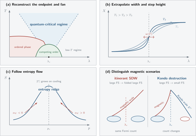
A material inference ledger. (a) A continuous $T=0$ endpoint can organize a finite-temperature fan, while competing order may hide the lowest-temperature approach. Dashed fan edges are crossovers. (b) A tuning curve may sharpen with cooling; both its width and limiting step height must be extrapolated. (c) when pressure is the tuning direction, entropy accumulation near $p_c$ produces opposite thermal-expansion signs on the two sides and a singular Grüneisen response under the stated scaling assumptions. (d) an itinerant spin-density-wave endpoint reconstructs an already large Fermi surface through broken translation symmetry, whereas Kondo destruction introduces a separate localization scale and a large-to-small Fermi-volume change. The panels are diagnostic schematics, not universal phase diagrams.

A fan can be hidden or truncated

Superconductivity, nematic order, charge order, or another low-temperature instability can preempt the putative endpoint. The normal state may then be accessed only by field, pressure, disorder, or extrapolation, each of which changes the Hamiltonian. A fan drawn through a competing phase is a hypothesis about an underlying normal state, not a directly observed region.

A first-order transition also has a broad finite-temperature fluctuation regime when its discontinuity is weak. Likewise, a narrow-band crossover can create a V-shaped map without any singular zero-temperature endpoint. The evidence must reach beyond the geometry of a color plot.

Scaling as a Material Test

Introduce the dimensionless temperature $t=k_{\mathrm B}T/E_0$. After subtracting an explicitly modeled regular contribution, a singular observable may take the form

$$X_s(r,T) = X_0 t^{\kappa_X} \Phi_X\!\left( \frac{r}{t^{1/(\nu z)}} \right).$$

The exponent $\kappa_X$ depends on the observable and on whether dangerously irrelevant variables or conservation laws modify naive hyperscaling. This equation is a testable ansatz, not permission to optimize every parameter until curves overlap.

Crossover sharpening

Suppose a field or pressure sweep shows a crossover of width $w_\lambda(T)$. Single-parameter scaling predicts, up to corrections,

$$\frac{w_\lambda(T)}{\lambda_0} = C_w t^{1/(\nu z)} \left[ 1+c_w t^{\omega/z}+\cdots \right],$$

where $\omega>0$ is a correction exponent. The center, width, step height, and background should be fitted separately. A width extrapolating to zero while the step height also vanishes does not establish a discontinuity in the zero-temperature observable.

Dynamical scaling

For a critical mode near wavevector $\mathbf Q$, define the thermal correlation length

$$\xi_T = \xi_0 t^{-1/z}.$$

A common dynamical test is

$$\chi''(\mathbf q,\omega,T) = \chi_0 t^{-a} \Phi_\chi\!\left( (\mathbf q-\mathbf Q)\xi_T, \frac{\hbar\omega}{k_{\mathrm B}T} \right).$$

An $\hbar\omega/(k_{\mathrm B}T)$ collapse is often called $E/T$ scaling. It is strongest when the same exponents describe several momenta and temperatures, instrumental resolution is folded into the fit, detailed balance is respected, and sum rules remain consistent. A collapse over less than a decade or after a temperature-dependent background subtraction is only suggestive.

A reproducible collapse protocol

1. Determine $\lambda_c$ from phase-boundary or thermodynamic data that are independent of the collapsed observable.
2. Fix the nonsingular background from a stated control window or a simultaneous global model.
3. Preserve the full covariance of data sharing contacts, calibration, normalization, or subtraction parameters.
4. Fit one scaling window, then test neighboring temperatures and detunings without refitting all parameters.
5. Compare against alternative exponents, polynomial crossover models, and a first-order or avoided-critical model.
6. Report drift with the fit window and the uncertainty in $\lambda_c$, not only the visually best collapse.

Probe	Critical information	Typical ambiguity
Calorimetry	entropy and singular free-energy derivatives	phonons, nuclear Schottky terms, addenda
Thermal expansion	pressure derivative of entropy	anisotropic stress, mounting, noncritical lattice background
Neutron or X-ray scattering	ordering wavevector, correlation length, $\omega/T$ scaling	resolution, form factors, limited energy window
NMR, NQR, μSR	local dynamics, static volume fraction, relaxation distribution	hyperfine filtering, disorder, field perturbation
Quantum oscillations	extremal areas and cyclotron masses	high fields, magnetic breakdown, disappearing amplitude
Hall and thermoelectric response	Fermi-surface-sensitive crossover	multiband weighting, anomalous Hall terms, skew scattering
Electrical and thermal transport	current relaxation and carrier integrity	cold-region short circuit, contacts, phonons, disorder

Entropy, Thermal Expansion, and Grüneisen Tests

A continuous endpoint concentrates low-energy states. At fixed nonzero temperature, the entropy often forms a ridge near the critical trajectory. This provides a thermodynamic diagnostic independent of a transport relaxation model.

The volume thermal-expansion coefficient obeys the Maxwell relation

$$\alpha_V = \frac{1}{V} \left( \frac{\partial V}{\partial T} \right)_p = -\frac{1}{V} \left( \frac{\partial S}{\partial p} \right)_T.$$

If pressure moves the system through an entropy maximum, $\alpha_V$ changes sign across the ridge. The critical pressure Grüneisen parameter may be written

$$\Gamma_p^{\mathrm{cr}} = \frac{V_m}{\kappa_T} \frac{\alpha_V^{\mathrm{cr}}}{C_p^{\mathrm{cr}}},$$

where $V_m$ is molar volume and $\kappa_T$ is isothermal compressibility. For a generic pressure-tuned endpoint governed by one leading relevant field,

$$\Gamma_p^{\mathrm{cr}}(p_c,T) \propto T^{-1/(\nu z)}.$$

Away from $p_c$, its low-temperature singular part commonly approaches a signed inverse detuning. These predictions require the critical pieces of both numerator and denominator, a known pressure coupling, and no more singular competing contribution. Anisotropic crystals can have different linear-expansion signs even when the volume response follows the expected entropy flow.

For a field-tuned endpoint, the magnetic Grüneisen parameter is

$$\Gamma_H = -\frac{(\partial M/\partial T)_H}{C_H} = \frac{1}{T} \left( \frac{\partial T}{\partial H} \right)_S.$$

It measures the magnetocaloric slope of an isentrope. A divergence and sign change near $H_c$ can locate entropy accumulation, but eddy-current heating, nuclear contributions, hysteresis, and finite sweep rate must be controlled.

Transport Anomalies: Powerful but Nonunique

A Landau Fermi liquid has an electronic resistivity that often approaches

$$\rho(T,\lambda) = \rho_0(\lambda) + A(\lambda)T^2$$

when electron–electron scattering dominates and momentum relaxation is available. Near many candidate endpoints, the empirical form

$$\rho(T,\lambda) = \rho_0(\lambda) + A_n(\lambda)T^{n(\lambda)}$$

has $n<2$, sometimes close to one. The local logarithmic slope

$$n_{\mathrm{eff}}(T) = \frac{\partial\ln[\rho(T)-\rho_0]}{ \partial\ln T }$$

is more informative than fitting one exponent across a broad crossover. Its uncertainty is dominated by the residual-resistivity estimate at the lowest temperatures.

Why the exponent is not universal

Transport weights momentum relaxation, velocities, Fermi-surface geometry, impurity mixing, and current vertices. In an itinerant antiferromagnetic scenario, critical scattering can be concentrated near hot spots joined by $\mathbf Q$, while cold regions conduct in parallel. Disorder can mix the two. Phonons, valence fluctuations, a nearby Lifshitz transition, two-level systems, and hydrodynamic flow can also produce nonquadratic laws.

Linear-$T$ resistivity is therefore a phenomenon to explain, not a standalone measurement of $z$ or proof of a quantum critical point. The canonical treatments of the Boltzmann and Kubo frameworks are Boltzmann Transport and Kubo Formula.

Charge versus heat

The Lorenz ratio is

$$L(T) = \frac{\kappa}{\sigma T}, \qquad L_0 = \frac{\pi^2k_{\mathrm B}^2}{3e^2}.$$

Testing the Wiedemann–Franz limit requires $T\to0$, the electronic thermal conductivity, matched electrical contacts, and subtraction or bounding of phonon, magnon, neutral-fermion, and nuclear heat channels. A finite-temperature deviation can reflect inelastic scattering even when charged quasiparticles survive asymptotically.

Optical conductivity adds frequency resolution. A proposed $\omega/T$ scaling or Planckian relaxation rate must state whether the response is Drude-like, which spectral weight and effective mass define the rate, how interband absorption was removed, and whether the sum rule is satisfied. A fitted $\hbar/\tau\sim k_{\mathrm B}T$ is not universal until those choices are controlled across systems.

Magnetic Quantum Criticality

Magnetic metals are especially revealing because order-parameter fluctuations coexist with gapless fermions. They are also especially difficult because integrating out those fermions can generate damping and nonlocal interactions.

Itinerant spin-density-wave endpoint

In the simplest antiferromagnetic Hertz–Millis description, the low-energy inverse susceptibility near the ordering vector has the schematic form

$$\chi^{-1}(\mathbf Q+\mathbf q,i\omega_n) = r + cq^2 + \gamma|\omega_n| + \cdots .$$

The damping gives $z=2$ in this common clean antiferromagnetic case. The order parameter reconstructs the Fermi surface by folding the Brillouin zone, but the electronic degrees of freedom counted in the paramagnetic heavy Fermi liquid need not localize. Critical scattering is strongest near hot regions connected by $\mathbf Q$.

This framework is not one formula for every magnet. Ferromagnetic fluctuations have different damping and couple to long-wavelength particle–hole modes. In clean metallic ferromagnets, nonanalytic fermionic corrections often drive the low-temperature transition first order or stabilize modulated order. A material with avoided ferromagnetic criticality should not be forced into the antiferromagnetic $z=2$ template.

Kondo destruction

In a heavy-fermion metal, magnetic order can coincide with the collapse of Kondo entanglement. A second low-energy scale $E^*$ then tends to zero, and the charged Fermi surface can change from a large count including the local moments to a small count excluding them. The critical theory contains more than fluctuations of the magnetic order parameter.

Candidate evidence includes a crossover in Hall or magnetostriction that sharpens on cooling, a Fermi-surface change not accounted for by ordinary zone folding, dynamical scaling with a strong local component, and the merger of the magnetic and Kondo-localization scales. None is decisive alone. Multiband Hall coefficients are not direct carrier counts, quantum-oscillation amplitudes can disappear because masses or scattering diverge, and finite-temperature crossover lines can detach from the magnetic boundary.

Scenario	Zero-temperature change	Material clues	Principal falsification pressure
Itinerant spin-density wave	onset of magnetic order within an itinerant Fermi surface	ordering-vector fluctuations, hot-region scattering, continuous zone folding	singular response far from $\mathbf Q$ or an unexplained Fermi-volume jump
Kondo destruction	magnetic criticality plus localization of moment degrees of freedom	extra $E^*$ scale, large-to-small Fermi-surface evidence, local dynamical component	persistence of one large Fermi count through the endpoint
Lifshitz or van Hove tuning	change of Fermi-surface topology without required collective criticality	band-edge crossing, thermopower and density-of-states anomalies	scaling tied to an independently established order-parameter endpoint
Disorder or Griffiths regime	broad distribution of local energy scales	sample dependence, rare-region tails, distributed relaxation	clean-limit convergence and homogeneous critical volume fraction
Preempted endpoint	intervening first-order or ordered phase	hysteresis, latent heat, split lines, phase coexistence	continuous scaling demonstrably extending below the proposed preemption

Representative Material Ledgers

The following examples are landmarks, not a list of universally settled classifications.

Material or family	Tuning and adjacent physics	What established its importance	Remaining qualification
CeCu$_{6-x}$Au$_x$	Au concentration tunes antiferromagnetism near $x\simeq0.1$	quasi-two-dimensional magnetic fluctuations and anomalous $E/T$ scaling	substitution disorder and the relation between local and ordering-vector dynamics
YbRh$_2$Si$_2$	small field suppresses weak antiferromagnetism	divergent thermodynamics and a Hall-related crossover sharpening toward the endpoint	multiband Hall interpretation and whether all low-energy lines terminate together
CeRhIn$_5$	pressure suppresses antiferromagnetism near superconductivity	strong mass enhancement and abrupt quantum-oscillation reconstruction	high-field access and superconductivity alter the route to the normal state
Sr$_3$Ru$_2$O$_7$	field and angle tune metamagnetic behavior	entropy and transport anomalies around a field-tuned endpoint	an electronic nematic phase preempts the simplest naked endpoint in clean samples
MnSi	pressure suppresses helimagnetism	extended non-Fermi-liquid transport and unusual magnetic correlations	the transition becomes first order, so the broad regime is not a simple continuous QCP fan
Spin-dimer magnets	field closes a singlet–triplet gap	comparatively direct bosonic critical modes and neutron access	anisotropy, magnetoelastic coupling, and dimensional crossover modify ideal condensation scaling

These cases illustrate why “proximity to a QCP” must specify the endpoint, tuning path, hidden or intervening phases, and observables. Similar transport exponents across two compounds do not by themselves imply the same universality class.

Material Inference Workflow

1. Identify the phases. Establish symmetry, excitations, Fermi-surface character, and volume fraction on both sides.
2. Calibrate the tuning field. Record pressure gradients, field orientation, composition distribution, strain tensor, or carrier-density conversion.
3. Determine transition order. Search for latent heat, hysteresis, coexistence, and protocol dependence down to the lowest temperature.
4. Map every low-energy line. Include ordering, superconducting, metamagnetic, Kondo-coherence, Fermi-surface, and structural crossovers.
5. Construct an entropy ledger. Integrate calibrated heat capacity and compare thermal-expansion or magnetocaloric flow.
6. Separate singular and regular pieces. State phonon, nuclear, impurity, anomalous-Hall, and multiband backgrounds.
7. Test scaling globally. Use one $\lambda_c$, shared exponents where theory requires them, correction terms, and held-out windows.
8. Compare mechanisms. Fit order-parameter, Kondo-destruction, Lifshitz, disorder, and first-order alternatives to discriminating observables.
9. Check sample and path dependence. Repeat across residual resistivity, field orientation, pressure medium, and at least one independent tuning direction where feasible.
10. State the limiting claim. Distinguish an observed finite-temperature regime from an inferred continuous $T=0$ endpoint and from a proposed microscopic fixed point.

Common Mistakes

• Calling every V-shaped finite-temperature map a quantum-critical fan.
• Extrapolating $T_{\mathrm{ord}}$ to zero without checking whether the transition remains continuous.
• Identifying $\lambda_c$ and exponents from the same optimized data collapse without propagating their covariance.
• Treating fan boundaries as thermodynamic phase boundaries.
• Assigning a universality class from one resistivity exponent.
• Calling every Hall crossover a carrier-density or Fermi-volume jump.
• Ignoring anomalous Hall terms, multiband mobilities, and skew scattering.
• Interpreting missing quantum oscillations as proof that a Fermi-surface sheet vanished.
• Applying a clean Hertz–Millis exponent to a disordered or ferromagnetic transition.
• Reading a divergent Grüneisen ratio without subtracting nuclear, phonon, or noncritical electronic terms.
• Claiming a Wiedemann–Franz violation from a finite-temperature extrapolation with unbounded neutral heat channels.
• Drawing a hidden endpoint beneath superconductivity as if it had been directly observed.
• Equating $\hbar/\tau\sim k_{\mathrm B}T$ with a universal microscopic mechanism.

Exercises

1. Infer a crossover exponent product

A field-sweep crossover has full width $w=0.24\,\mathrm T$ at $8\,\mathrm K$ and $w=0.12\,\mathrm T$ at $2\,\mathrm K$. Assuming $w\propto T^{1/(\nu z)}$ and negligible corrections, infer $\nu z$.

Solution

The ratios obey

$$\frac{0.12}{0.24} = \left( \frac{2}{8} \right)^{1/(\nu z)}.$$

Thus

$$\frac{1}{2} = \left( \frac{1}{4} \right)^{1/(\nu z)},$$

which gives $1/(\nu z)=1/2$ and therefore $\nu z=2$.

This two-point estimate is not a publishable exponent determination. A real analysis needs more temperatures, uncertainty in the width and center, correction terms, and a test that the step shape is governed by one scaling function.

2. Determine the thermal-expansion sign

At fixed low temperature, the entropy $S(p)$ rises as pressure approaches $p_c$ from below and falls after passing through a maximum. What signs of $\alpha_V$ are expected on the two sides?

Solution

Use

$$\alpha_V = -\frac{1}{V} \left( \frac{\partial S}{\partial p} \right)_T.$$

Below $p_c$, $(\partial S/\partial p)_T>0$, so $\alpha_V<0$. Above $p_c$, the entropy decreases with pressure, so $(\partial S/\partial p)_T<0$ and $\alpha_V>0$. The sign change points toward the entropy ridge.

The argument concerns the singular volume response. A measured linear expansion along one axis can have another sign because uniaxial stress couples differently, and a regular lattice background can mask the critical contribution.

3. Can linear resistivity locate the endpoint?

A sample has $\rho=\rho_0+AT$ from $0.8$ to $8\,\mathrm K$ at one pressure. No phase boundary, heat capacity, or pressure sweep is reported. What can be concluded?

Solution

The data establish a linear-resistivity window after accepting the fitted $\rho_0$. They do not locate a zero-temperature endpoint or identify its universality class. Phonons, disorder, multiple bands, valence fluctuations, a nearby band-topology change, or an extended incoherent regime can produce a similar law.

A quantum-critical claim needs a pressure-resolved phase diagram, evidence that a continuous transition approaches zero, a shrinking detuning scale, and independent thermodynamic or dynamical consistency. Varying residual resistivity and extending to lower temperature would test whether cold regions, disorder, or another asymptotic regime change the exponent.

4. Extrapolate a Hall crossover carefully

A Hall-related observable is fitted by

$$R_H(H,T) = R_<(T) + \Delta R(T) f\!\left( \frac{H-H^*(T)}{w(T)} \right),$$

where $f$ is a smooth step. Measurements find $w(T)\to0$ and $\Delta R(T)\to\Delta R_0\ne0$ as $T\to0$. What is the strongest immediate inference, and what remains to be checked?

Solution

Within the fitted family and extrapolation window, the result supports a discontinuity of this Hall-related observable at $H^*(0)$. It is stronger than observing a sharpening slope because the limiting step height remains finite.

It is not yet a model-independent measurement of Fermi volume. One must bound anomalous Hall and skew-scattering terms, account for multiband mobilities, verify that the sample temperature follows the bath during field sweeps, and show that $H^*(0)$ coincides with or has a controlled relation to the thermodynamic endpoint. Quantum oscillations, magnetostriction, and spectroscopy can test the Fermi-surface interpretation.

5. Hot and cold regions in parallel

Suppose a simplified metal has independent hot and cold conduction channels with

$$\sigma_h = \frac{C_h}{T}, \qquad \sigma_c = \frac{C_c}{T^2},$$

and $C_h,C_c>0$. Find the low-temperature power of the total resistivity $\rho=1/(\sigma_h+\sigma_c)$.

Solution

The total conductivity is

$$\sigma = \frac{C_hT+C_c}{T^2}.$$

Therefore

$$\rho = \frac{T^2}{C_c+C_hT} \xrightarrow[T\to0]{} \frac{T^2}{C_c}.$$

The cold channel short-circuits the hot channel asymptotically, even though the hot contribution alone has linear resistivity. This toy result explains why a scattering-rate exponent at critical hot spots need not equal the measured bulk resistivity exponent. Impurities and vertex corrections can mix the regions and change the conclusion.

6. Design a field-tuned endpoint test

A magnetic insulator shows a broad heat-capacity maximum that moves to lower temperature with field and vanishes near $H_c$. Design a minimal test that separates a continuous field-tuned quantum critical point from a Schottky crossover or weak first-order transition.

Solution

First identify the two zero-temperature phases with symmetry-sensitive probes and measure the ordering line, not only the broad maximum. Calorimetry and magnetization sweeps should test latent heat, hysteresis, and coexistence while sweep-rate and magnetocaloric effects are controlled.

Next measure the excitation gap by spectroscopy on both sides and test whether it closes at the same $H_c$. Map the crossover width versus temperature, measure the magnetic Grüneisen parameter with nuclear and phonon terms bounded, and test one scaling form with $H_c$ fixed independently. A Schottky anomaly should track a finite-level splitting and need not produce a diverging correlation length, ordering susceptibility, or consistent gap closure. Repetition at several sweep rates and on warming and cooling constrains a weak first-order transition.

Research Status and Open Problems

Several elements are standard: continuous zero-temperature endpoints generate vanishing detuning scales; finite-temperature fan edges are crossovers; thermodynamic Grüneisen responses are singular under generic single-field scaling; and gapless fermions make metallic magnetic criticality more intricate than an isolated bosonic order parameter.

The following questions remain active:

• Which metallic antiferromagnetic endpoints flow to Hertz–Millis behavior, and which retain critical fermions that invalidate integrating them out?
• When does Kondo destruction coincide with magnetic ordering, and when do the two boundaries separate?
• What microscopic processes produce robust linear-$T$ resistivity and frequency-over-temperature charge scaling across heavy fermions, cuprates, iron-based materials, and moiré systems?
• Is a Planckian-looking rate a universal property, a transport bound, or an observable-dependent parametrization?
• How do rare regions and random strain alter apparent exponents in composition-tuned materials?
• How should superconductivity nucleated near a critical metal be separated from, and used to diagnose, the hidden normal state?
• Can quantum Fisher information, ultrafast spectroscopy, noise, and momentum-resolved probes distinguish critical entanglement from broad incoherence?
• Which sign-problem-free or otherwise controlled numerical models reproduce the coupled scaling of thermodynamics, single-particle spectra, and charge transport seen in materials?

Recent tunable Kondo platforms and improved stress, calorimetric, terahertz, and spatially resolved probes expand the available tests. They do not remove the need for conservative language: many materials are demonstrably near a zero-temperature instability, while the universality class and microscopic critical degrees of freedom remain unsettled.

Connections

• Quantum Phase Transitions owns the general zero-temperature definition, fan construction, and benchmark scaling.
• Critical Exponents and Scaling develops exponent identities, correction terms, finite-size collapse, and uncertainty practice.
• Heat Capacity and Thermodynamics owns calorimeter models, regular and singular background separation, entropy integration, and nuclear or Schottky controls.
• Kondo Lattices owns the dense Hamiltonians, Doniach heuristic, heavy-Fermi-liquid count, and Kondo-breakdown phase vocabulary.
• Heavy Fermions owns the representative compounds, effective-mass ledger, coherence evidence, and superconducting phenomenology.
• Competing Orders owns coupled finite-temperature phase topology, coexistence criteria, and the distinction between nearby phases and a demonstrated zero-temperature endpoint.
• Non-Fermi Liquids owns the quasiparticle-failure tests, self-energy classification, transport caveats, and replacement-mechanism map.
• Strange Metals owns the cross-material evidence for linear-$T$ resistivity, Planckian rate extractions, and multi-probe transport mechanisms.
• Itinerant Magnetism develops Stoner response, spin-density waves, paramagnons, and band-electron magnetic order.
• Antiferromagnetism owns Néel order, magnetic wavevectors, spin flop, and material diagnostics.
• Susceptibilities fixes source conventions, analytic continuation, static limits, and matrix eigenchannels.
• Disorder in Quantum Matter supplies the ensemble, correlator, lifetime, and sample-control ledger needed before invoking Griffiths physics.
• Kubo Formula owns exact linear response, contact terms, and transport limits.
• Critical Phenomena and RG Bridge connects material scaling observables to continuum operators and fixed points.

References

• J. A. Hertz, “Quantum critical phenomena,” Physical Review B 14, 1165–1184 (1976).
• A. J. Millis, “Effect of a nonzero temperature on quantum critical points in itinerant fermion systems,” Physical Review B 48, 7183–7196 (1993).
• T. Moriya and T. Takimoto, “Anomalous properties around magnetic instability in heavy electron systems,” Journal of the Physical Society of Japan 64, 960–969 (1995).
• N. D. Mathur, F. M. Grosche, S. R. Julian, et al., “Magnetically mediated superconductivity in heavy fermion compounds,” Nature 394, 39–43 (1998).
• O. Stockert, H. v. Löhneysen, A. Rosch, N. Pyka, and M. Loewenhaupt, “Two-dimensional fluctuations at the quantum-critical point of CeCu$_{6-x}$Au$_x$,” Physical Review Letters 80, 5627–5630 (1998).
• A. Schröder, G. Aeppli, R. Coldea, et al., “Onset of antiferromagnetism in heavy-fermion metals,” Nature 407, 351–355 (2000).
• G. R. Stewart, “Non-Fermi-liquid behavior in $d$- and $f$-electron metals,” Reviews of Modern Physics 73, 797–855 (2001).
• S. A. Grigera, R. S. Perry, A. J. Schofield, et al., “Magnetic field-tuned quantum criticality in the metallic ruthenate Sr$_3$Ru$_2$O$_7$,” Science 294, 329–332 (2001).
• Q. Si, S. Rabello, K. Ingersent, and J. L. Smith, “Locally critical quantum phase transitions in strongly correlated metals,” Nature 413, 804–808 (2001).
• L. Zhu, M. Garst, A. Rosch, and Q. Si, “Universally diverging Grüneisen parameter and the magnetocaloric effect close to quantum critical points,” Physical Review Letters 91, 066404 (2003).
• R. Küchler, N. Oeschler, P. Gegenwart, et al., “Divergence of the Grüneisen ratio at quantum critical points in heavy fermion metals,” Physical Review Letters 91, 066405 (2003).
• J. Custers, P. Gegenwart, H. Wilhelm, et al., “The break-up of heavy electrons at a quantum critical point,” Nature 424, 524–527 (2003).
• S. Paschen, T. Lühmann, S. Wirth, et al., “Hall-effect evolution across a heavy-fermion quantum critical point,” Nature 432, 881–885 (2004).
• D. Belitz, T. R. Kirkpatrick, and T. Vojta, “How generic scale invariance influences quantum and classical phase transitions,” Reviews of Modern Physics 77, 579–632 (2005).
• H. v. Löhneysen, A. Rosch, M. Vojta, and P. Wölfle, “Fermi-liquid instabilities at magnetic quantum phase transitions,” Reviews of Modern Physics 79, 1015–1075 (2007).
• R. A. Borzi, S. A. Grigera, J. Farrell, et al., “Formation of a nematic fluid at high fields in Sr$_3$Ru$_2$O$_7$,” Science 315, 214–217 (2007).
• P. Gegenwart, Q. Si, and F. Steglich, “Quantum criticality in heavy-fermion metals,” Nature Physics 4, 186–197 (2008).
• S. Sachdev and B. Keimer, “Quantum criticality and the fate of the Fermi liquid in high-temperature superconductors,” Nature Physics 7, 74–78 (2011).
• M. Brando, D. Belitz, F. M. Grosche, and T. R. Kirkpatrick, “Metallic quantum ferromagnets,” Reviews of Modern Physics 88, 025006 (2016).
• L. Prochaska, X. Li, D. C. MacFarland, et al., “Singular charge fluctuations at a magnetic quantum critical point,” Science 367, 285–288 (2020).
• S. Paschen and Q. Si, “Quantum phases driven by strong correlations,” Nature Reviews Physics 3, 9–26 (2021).
• W. Zhao, B. Shen, Z. Tao, et al., “Gate-tunable heavy fermions in a moiré Kondo lattice,” Nature 616, 61–65 (2023).
• H. Hu, L. Chen, and Q. Si, “Quantum critical metals and loss of quasiparticles,” Nature Physics 20, 1863–1873 (2024).

Summary

Quantum criticality in a material is an inference about a continuous zero-temperature endpoint and the finite-temperature, finite-frequency scales it organizes. The strongest case identifies both phases, verifies that the transition remains continuous, reconstructs shrinking crossover scales, and makes thermodynamics, dynamics, Fermi-surface-sensitive probes, and transport agree on one critical trajectory. Fan geometry, linear resistivity, a Hall crossover, or an $E/T$ plot is not sufficient alone. Metallic magnets sharpen the challenge because order-parameter fluctuations, gapless fermions, Kondo entanglement, disorder, and competing phases can all reorganize the same observables. Trustworthy claims therefore state the tuning path, backgrounds, limiting procedures, alternatives, and unresolved microscopic status.