Emergent Gauge Fields

An emergent gauge field is a collective low-energy degree of freedom whose gauge structure arises from the constrained Hilbert space and dynamics of a many-body system. It is not inserted as a fundamental interaction. Its electric charges, flux defects, photons, and confinement scales are encoded in gauge-invariant properties of the original spins, electrons, atoms, or qubits.

The phrase contains two logically separate claims:

1. A useful low-energy description has a local redundancy. Different auxiliary-field configurations label the same physical state.
2. Fluctuations associated with that redundancy have dynamics and survive over a controlled energy and length window. Depending on dimension and matter content, they may form a deconfined Coulomb phase, a gapped discrete gauge phase, a critical state, or a confined regime.

A parton decomposition establishes the first claim, not the second. Conversely, a Berry connection, an applied electromagnetic potential, or a smoothly varying magnetic texture can be called a gauge field in other contexts without constituting an emergent deconfined gauge sector. The decisive questions are what enforces the Gauss law, what carries gauge charge and flux, and what gauge-invariant measurement tests the resulting theory.

Canonical Scope

This page is the canonical home for the physical emergence and many-body consequences of dynamical gauge fields in quantum matter. It owns:

• the route from local constraints and redundant variables to a lattice Gauss law;
• compact U(1), $\mathbb Z_2$, and non-Abelian gauge structures in spin liquids;
• confinement, Coulomb, and Higgs regimes, including their dimensional qualifications;
• coupling between gauge fields and Dirac spinons or spinon Fermi surfaces;
• a gauge-invariant evidence standard for materials and quantum simulators.

Phase, Symmetry, and Gauge Theory owns the broader conceptual bridge among phases, global symmetries, background fields, and dynamical gauge fields. Fractionalization owns the local-sector and deconfinement criteria for the matter excitations. Quantum Spin Liquids owns the phase taxonomy and candidate-material ledger. Topological Order and Anyons and Braiding own universal anyon, loop-algebra, modular, and braiding data. Formal gauge fixing, ghosts, perturbative renormalization, and fundamental Yang–Mills dynamics belong in quantum field theory.

From a Constraint to Gauss’s Law

Redundant variables are not extra physical states

For a spin-$1/2$ moment, introduce fermionic partons $f_{i\alpha}$ through

$$\mathbf S_i = \frac{1}{2} f_{i\alpha}^{\dagger} \boldsymbol\sigma_{\alpha\beta} f_{i\beta}, \qquad n_i^f = \sum_\alpha f_{i\alpha}^{\dagger}f_{i\alpha} =1.$$

Every spin operator is unchanged by the site-dependent transformation

$$f_{i\alpha}\longmapsto e^{i\theta_i}f_{i\alpha}.$$

This local U(1) is a redundancy introduced by enlarging the two-dimensional spin Hilbert space to a fermionic Fock space. The constraint $n_i^f=1$ projects back to physical states. A mean-field expectation value such as $\langle f_i^\dagger f_j\rangle$ is gauge dependent and therefore cannot itself be an observable order parameter.

In a path integral, a Lagrange multiplier enforces the constraint:

$$S_{\mathrm{con}} = \int d\tau\, \sum_i i a_{0,i}(n_i^f-1).$$

A bond decoupling can be parameterized as

$$\chi_{ij}=|\chi_{ij}|e^{ia_{ij}}.$$

Under the local rephasing, the phases transform as

$$\begin{aligned} a_{ij}&\longmapsto a_{ij}+\theta_i-\theta_j,\\ a_{0,i}&\longmapsto a_{0,i}+\partial_\tau\theta_i. \end{aligned}$$

The temporal multiplier and fluctuating bond phase therefore assemble into a lattice gauge connection. Whether these fluctuations are deconfined, massive, or confining is a dynamical question that must be answered after the constraint has been imposed.

Constrained configurations give a more direct route

Quantum dimer models and spin ice expose the same structure without beginning from an arbitrary factorization. Orient the links of a lattice and assign an integer or half-integer electric field $E_\ell$ to each link. A local rule on allowed dimers or spins becomes

$$(\nabla\cdot E)_r \equiv \sum_{\ell\ni r}\eta_{r\ell}E_\ell = \rho_r,$$

where $\eta_{r\ell}=+1$ for an outgoing link and $-1$ for an incoming link. The background or defect charge $\rho_r$ is fixed by the microscopic rule. In spin ice, the two-in/two-out condition is a divergence-free law after a conventional background subtraction; a violated tetrahedron carries emergent gauge charge.

The logic is structural:

$$\text{local constraint} \quad\Longrightarrow\quad \text{Gauss-law sector} \quad\Longrightarrow\quad \text{gauge-compatible dynamics}.$$

Not every constraint produces a useful long-wavelength gauge field. The constrained manifold must be extensive, local moves must connect its sectors, and quantum dynamics must generate coherent fluctuations before defects or ordering destroy the description.

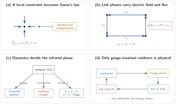
The inference chain for an emergent gauge field. A local microscopic rule supplies Gauss’s law; compact link variables carry conjugate electric field and plaquette flux; monopoles and charged condensates select Coulomb, confined, $\mathbb Z_2$, or Higgs regimes; and the final claim must close using observables invariant under the redundancy.

Compact U(1) Dynamics

Link variables and the lattice Hamiltonian

Place a periodic phase $a_\ell\equiv a_\ell+2\pi$ on each oriented link and its conjugate electric field $E_\ell$ on the same link:

$$[a_\ell,E_{\ell'}] = i\delta_{\ell\ell'}.$$

The minimal compact U(1) Hamiltonian is

$$H_{\mathrm{gauge}} = \frac{U}{2}\sum_\ell E_\ell^2 -K\sum_p \cos\!\left[(\nabla\times a)_p\right],$$

restricted by $(\nabla\cdot E)_r=\rho_r$. The first term penalizes electric flux. The second resonates flux around a plaquette $p$. Compactness matters: the plaquette flux is defined modulo $2\pi$, so topological events that change flux by $2\pi$ are allowed.

The unitary operator generated by the Gauss constraint,

$$G[\theta] = \exp\!\left[ i\sum_r\theta_r \bigl((\nabla\cdot E)_r-\rho_r\bigr) \right],$$

acts trivially on physical states. It shifts $a_{rr'}$ by $\theta_r-\theta_{r'}$ and rephases matter of gauge charge one. Gauge invariance is thus the operator statement that the dynamics preserves the constrained physical subspace.

The Coulomb phase and emergent photon

When flux fluctuations remain small, expand the cosine and coarse-grain. In three spatial dimensions the leading continuum Hamiltonian has Maxwell form,

$$H_{\mathrm{Maxwell}} = \frac{1}{2} \int d^3x\, \left( \epsilon^{-1}\mathbf E^2 + \mu^{-1}\mathbf B^2 \right), \qquad \mathbf B=\nabla\times\mathbf a.$$

Transverse fluctuations then obey

$$\omega_{\mathbf q}=c_{\mathrm e}|\mathbf q|+mathcal O(q^3), \qquad c_{\mathrm e}=\frac{1}{\sqrt{\epsilon\mu}}.$$

This emergent photon is a neutral collective mode of the medium. Its velocity $c_{\mathrm e}$ is set by microscopic exchange scales and lattice spacing, not by the vacuum speed of light. Gauge charges and magnetic monopoles are separate excitations, generally gapped in a three-dimensional quantum spin ice.

For one linearly dispersing photon with two transverse polarizations in three dimensions, the low-temperature energy density and heat capacity scale as

$$\frac{U_\gamma}{V} = \frac{\pi^2}{15} \frac{(k_{\mathrm B}T)^4} {\hbar^3c_{\mathrm e}^3}, \qquad \frac{C_\gamma}{V} = \frac{4\pi^2}{15} \frac{k_{\mathrm B}^4T^3} {\hbar^3c_{\mathrm e}^3}.$$

The $T^3$ law is not distinctive by itself because acoustic phonons have the same power. A credible assignment needs the coefficient, momentum and polarization structure, field evolution, and a phonon baseline.

Compactness, monopoles, and dimension

The noncompact Maxwell theory omits tunneling events between flux sectors. In a compact theory, monopole or instanton operators insert quantized flux. Their infrared relevance depends on spacetime dimension, matter content, and microscopic symmetries.

• Pure compact U(1) gauge theory in $2+1$ dimensions confines at long distance through monopole proliferation.
• Compact U(1) gauge theory can have a stable deconfined Coulomb phase in $3+1$ dimensions, with a photon and gapped electric and magnetic charges.
• Gapless matter can suppress monopoles in $2+1$ dimensions. Large-flavor compact QED$_3$ supplies a controlled deconfined limit, but stability at the small physical flavor number is model and symmetry dependent.
• A lattice distortion or another symmetry-allowed perturbation can couple directly to monopole operators and destabilize a proposed U(1) Dirac spin liquid.

Writing a Maxwell action is therefore not enough. One must specify whether the gauge field is compact and list every symmetry-allowed monopole perturbation.

Discrete and Non-Abelian Gauge Structures

From U(1) to ℤ₂

Let a charge-two field $\Phi$ couple to a U(1) gauge field:

$$\mathcal L_\Phi = \left|\left(\partial_\mu-2ia_\mu\right)\Phi\right|^2 +V(|\Phi|) +\frac{1}{4e^2}f_{\mu\nu}f^{\mu\nu}.$$

In the Higgs regime where the amplitude of $\Phi$ is nonzero, transformations with $e^{2i\theta}=1$ leave the condensate representative unchanged. The surviving low-energy gauge structure is $\mathbb Z_2$. Its deconfined phase in $2+1$ dimensions has gapped gauge charge, gapped flux called a vison, and no gapless photon. The charge and vison have nontrivial mutual statistics, as developed on Topological Order.

One should not say that a local gauge symmetry spontaneously breaks. Elitzur’s theorem forbids a gauge-noninvariant local expectation value from serving as a physical order parameter. “Higgs regime” refers to a gauge-invariant change in spectrum and long-distance response. With matter in a fundamental representation, nominal confinement and Higgs regions may even be analytically connected; the phase diagram must be established from the actual matter representation and global symmetries.

Loop diagnostics and their caveats

For a closed contour $C$, the Wilson loop is

$$W(C) = \left\langle \exp\!\left(i\sum_{\ell\in C}a_\ell\right) \right\rangle.$$

In a pure gauge theory, an area law $-\ln W(C)\propto A(C)$ indicates a string tension and confinement, while a perimeter law is compatible with deconfinement. A dual ’t Hooft loop inserts magnetic flux and reverses the electric-magnetic diagnosis.

These statements need a matter caveat. Dynamical fundamental charges can screen external probes and break a long string, converting an asymptotic Wilson-loop area law into a perimeter-like form even in a confining regime. Finite-size numerics should therefore combine loop behavior with flux-sector splittings, charge-pair energetics, string breaking, and the excitation spectrum.

Non-Abelian cases

A single spin representation may have a larger microscopic redundancy than its low-energy gauge structure. SU(2) parton formulations of a spin-$1/2$ system can be Higgsed to U(1) or $\mathbb Z_2$ by a particular ansatz. The physically relevant gauge group is the subgroup that leaves the ansatz invariant, together with the fluctuations that remain dynamical after high-energy modes are integrated out.

Deconfined non-Abelian gauge fields in $2+1$-dimensional magnets are more delicate than the familiar $\mathbb Z_2$ case. Pure Yang–Mills dynamics is confining; gapless matter or topological terms can qualitatively change the infrared theory. A Chern–Simons gauge theory can encode non-Abelian anyons without supplying a Maxwell-like propagating photon, so “non-Abelian anyons” and “gapless non-Abelian gauge bosons” are not synonyms.

The Kitaev honeycomb model illustrates another useful distinction. Its exact solution contains a $\mathbb Z_2$ gauge field. In a time-reversal-breaking gapped regime, the mobile Majorana sector supports non-Abelian Ising anyons. The gauge field itself has not become an SU(2) field merely because the anyon fusion rules are non-Abelian.

Infrared structure	Gauge mode	Characteristic excitations	Central stability issue
U(1) Coulomb phase in $3+1$D	Gapless photon	Electric charges and magnetic monopoles	Stability against charge or monopole condensation
U(1) Dirac state in $2+1$D	Strongly coupled to Dirac matter	Spinons and monopole operators	Flavor number, symmetry quantum numbers, lattice coupling
$\mathbb Z_2$ deconfined phase in $2+1$D	Gapped	Gauge charge, vison, and their bound state	Closing of charge or vison gap
Higgs regime	Usually massive	Spectrum depends on condensed charge	Matter representation and gauge-invariant phase distinction
Non-Abelian topological phase	Usually no local gapless gauge mode	Non-Abelian anyons	Gap, topological sector, and symmetry stability

Coupling to Fractionalized Matter

Dirac spinons and compact QED₃

A common continuum theory for a two-dimensional Dirac spin liquid is

$$\mathcal L_{\mathrm{QED}_3} = \sum_{a=1}^{N_f} \bar\psi_a\gamma^\mu (\partial_\mu-ia_\mu)\psi_a + \frac{1}{4e^2}f_{\mu\nu}f^{\mu\nu} + \mathcal L_{\mathrm{mon}}.$$

The fermions $\psi_a$ carry emergent gauge charge but need not carry electrical charge. Physical spin operators are gauge-neutral fermion bilinears or monopole operators. Their lattice momentum, spin, and point-group quantum numbers depend on the parton ansatz and its projective symmetry implementation.

The term $\mathcal L_{\mathrm{mon}}$ is not optional bookkeeping. It contains monopole insertions allowed by microscopic symmetries. If every allowed monopole is irrelevant, an algebraic spin liquid can persist. If an allowed monopole is relevant, its proliferation can confine spinons and often select Néel or valence-bond order. A continuum scaling analysis must therefore be matched to the microscopic symmetry quantum numbers.

A spinon Fermi surface

A finite density of gauge-charged fermions Landau damps the transverse U(1) gauge field. In a two-dimensional patch description,

$$D_T^{-1}(\mathbf q,\omega) \sim \chi q^2 + \gamma\frac{|\omega|}{|q_\parallel|},$$

where $q_\parallel$ is tangent to the local Fermi-surface patch. The corresponding fermion self-energy has the patch-scaling form

$$\Sigma(i\omega) \sim i\,\operatorname{sgn}(\omega) |\omega|^{2/3}.$$

Because $|\Sigma|/|\omega|$ grows at low frequency, the Landau quasiparticle is not asymptotically sharp. This is a canonical mechanism for a Non-Fermi Liquid, but numerical coefficients, transport exponents, and even controlled extrapolation can be subtle. Momentum relaxation, disorder, gauge-neutral sectors, and possible pairing of spinons must be treated separately.

Gauge charge is not laboratory charge

An emergent gauge charge labels the response to $a_\mu$; electric charge labels the response to the physical electromagnetic field $A_\mu$. A spinon may be electrically neutral and gauge charged, while a chargon may carry both. Only gauge-neutral combinations are locally creatable in the bulk.

This distinction is why response rules for parton sectors are constrained rather than simply additive. The Ioffe–Larkin composition rule and its assumptions are developed on Fractionalization; the present page does not duplicate that transport derivation.

Experimental Implications

No apparatus measures a gauge-dependent potential $a_\mu$ directly. Neutrons, photons, electrons, and thermodynamic probes couple to gauge-invariant operators of the microscopic system. The experimental task is to show that several such observables are governed by one constrained gauge theory.

Probe	Gauge-theory expectation	Necessary control
Elastic diffuse scattering	Pinch-point tensor structure from $\nabla\cdot\mathbf E=0$	Classical spin ice and resolution broadening can produce similar patterns
Inelastic neutron scattering	Photon-like low-energy weight and multi-spinon continuum	Phonons, magnons, disorder, and subtraction protocol
Heat capacity	$C_\gamma\propto T^3$ for a three-dimensional linear photon	Acoustic-phonon coefficient and nuclear Schottky terms
Field tuning	Different evolution of photon and gauge-charge sectors	Zeeman polarization, ordinary mode shifts, and hysteresis
Spectral threshold	Pair creation and gauge-dressed line shape	Conventional two-particle decay and parameter overfitting
Quantum simulation	Open strings create endpoints; closed loops diagnose flux and topology	Gauss-law fidelity, readout errors, boundaries, and finite size

Quantum spin ice

In a pyrochlore spin ice, the coarse-grained ice rule gives a divergence-free field and pinch points in the static structure factor. Those pinch points establish a Coulomb constraint, not by themselves a quantum photon: classical spin ice has them too. Quantum ring exchange can promote the constrained manifold to a U(1) quantum spin liquid with an emergent photon, gapped spinons carrying electric gauge charge, and gapped magnetic monopoles.

The strongest material strategy separates predicted sectors under a controlled perturbation. Experiments on Pr$_2$Hf$_2$O$_7$ reported quantum-modified pinch-point correlations and inelastic weight consistent with emergent electrodynamics. Spectroscopy of Ce$_2$Sn$_2$O$_7$ reported a gapped threshold and multiple peaks fitted by pair production of fractional matter in a $\pi$-flux gauge background. In 2026, field-dependent neutron work on Ce$_2$Zr$_2$O$_7$ reported that a weak [111] field suppresses low-energy photon weight while a higher-energy spinon continuum persists and hardens. These are substantial, increasingly specific tests, but each material assignment still depends on exchange calibration, disorder control, polarization, and the uniqueness of the model fit.

A disciplined evidence ladder

A mature claim should close four loops:

1. Constraint: microscopic interactions produce the proposed Gauss-law manifold over a measured energy range.
2. Charge and flux: distinct excitations have the thresholds, quantum numbers, and field response predicted for gauge charge and gauge flux.
3. Dynamics: a photon, gapped discrete gauge sector, or matter-damped propagator has the predicted momentum and frequency structure.
4. Alternatives: phonons, magnons, multiparticle decay, disorder, freezing, and subtraction artifacts are quantitatively bounded.

A broad continuum completes none of these steps on its own. Structure Factors develops the sum rules and tensor information needed to compare neutron data with a microscopic operator.

Quantum simulators

Programmable atom and qubit arrays can prepare constrained Hamiltonians and measure observables unavailable in bulk materials. In a $\mathbb Z_2$ realization, an open string can create charge or flux defects at its endpoints, while a closed string probes loop response and topological sectors. Experiments have prepared toric-code-like states and measured nonlocal correlations consistent with topological spin-liquid structure.

Simulation does not remove the burden of verification. The implemented Hamiltonian, Gauss-law violation rate, finite-size gap, boundary conditions, adiabatic preparation error, and readout correction must all be reported. Demonstrating an engineered gauge theory is a controlled realization of the model, not evidence that a particular solid realizes the same phase. Ultracold-Atom Quantum Simulation develops the broader validation logic.

Common Mistakes

Treating redundancy as an ordinary symmetry

Gauge-related parton configurations are the same physical state. They are not distinct vacua connected by a physical operation. Use gauge-invariant spectra, loops, flux sectors, and composite correlators; do not assign meaning to a bare parton expectation value.

Declaring deconfinement at mean field

A saddle point may contain free spinons and a gapless gauge field while compact fluctuations confine the exact theory. Check monopoles, matter content, dimension, and every symmetry-allowed perturbation.

Calling every geometric connection emergent electromagnetism

A Berry connection is a connection over parameter or momentum space, and a spin-texture field may act as an effective magnetic field for adiabatic electrons. These are valuable structures, but neither automatically supplies a dynamical Gauss law, independent gauge-charge sector, and propagating gauge mode. See Berry Connection for the geometric object.

Equating a pinch point with a photon

A pinch point diagnoses an approximately divergence-free constraint. A quantum photon additionally requires low-energy dynamics with the predicted dispersion, polarization, temperature dependence, and field evolution.

Saying gauge symmetry spontaneously breaks

Gauge symmetry is redundancy. Describe a Higgs regime, charge condensation in a fixed gauge, or a change in gauge-invariant spectrum. Then state whether the Higgs and confinement regimes are sharply distinct in the specific theory.

Confusing non-Abelian anyons with non-Abelian photons

Non-Abelian fusion and braiding can emerge in a fully gapped topological phase. They do not imply a gapless Yang–Mills field in the material.

Exercises

1. Derive the gauge transformation of a bond field

Let $\chi_{ij}\propto\langle f_i^\dagger f_j\rangle=|\chi_{ij}|e^{ia_{ij}}$. Under $f_i\mapsto e^{i\theta_i}f_i$, find the transformation of $a_{ij}$ and show that the oriented plaquette flux is invariant.

Solution

The bilinear transforms as

$$f_i^\dagger f_j \longmapsto e^{-i\theta_i}e^{i\theta_j} f_i^\dagger f_j.$$

With the convention used in the text, this is equivalent to $a_{ij}\mapsto a_{ij}+\theta_i-\theta_j$ after reversing the orientation used for the mean-field hopping term. Around an oriented plaquette,

$$\Phi_p = \sum_{(ij)\in\partial p}a_{ij}.$$

Every site phase appears once with each sign, so the shifts telescope and $\Phi_p\mapsto\Phi_p$ modulo $2\pi$. The individual link phase is redundant; the loop flux is gauge invariant.

2. Count the emergent-photon heat capacity

Assume an isotropic three-dimensional U(1) Coulomb phase with dispersion $\omega=c_{\mathrm e}q$ and two transverse polarizations. Derive the low-temperature heat-capacity density.

Solution

The energy density is

$$\frac{U}{V} = 2\int\frac{d^3q}{(2\pi)^3} \frac{\hbar c_{\mathrm e}q} {e^{\beta\hbar c_{\mathrm e}q}-1}.$$

Using $x=\beta\hbar c_{\mathrm e}q$ and $\int_0^\infty dx\,x^3/(e^x-1)=\pi^4/15$ gives

$$\frac{U}{V} = \frac{\pi^2}{15} \frac{(k_{\mathrm B}T)^4} {\hbar^3c_{\mathrm e}^3}.$$

Differentiation yields

$$\frac{C}{V} = \frac{4\pi^2}{15} \frac{k_{\mathrm B}^4T^3} {\hbar^3c_{\mathrm e}^3}.$$

The same power as an acoustic phonon makes the coefficient and independent spectroscopic checks essential.

3. Higgs U(1) to ℤ₂

A field of gauge charge $q$ has nonzero amplitude in a Higgs regime. Which transformations leave its representative unchanged? Specialize to $q=2$ and identify the residual group.

Solution

The field transforms as $\Phi\mapsto e^{iq\theta}\Phi$. A fixed nonzero representative is unchanged when

$$q\theta=2\pi n, \qquad n\in\mathbb Z.$$

Thus the residual transformations are $\theta=2\pi n/q$, forming $\mathbb Z_q$. For $q=2$, the two elements are $\theta=0$ and $\pi$, so the low-energy gauge structure is $\mathbb Z_2$. This gauge-fixed argument predicts the spectrum; physical phase distinctions must still be stated through gauge-invariant quantities.

4. Why a Wilson loop can lose its area law

Suppose a confining string has tension $\sigma$ but the theory contains a dynamical charge-anticharge pair of mass $m$. Estimate the separation at which string breaking becomes favorable and explain the Wilson-loop caveat.

Solution

An unbroken string of length $R$ costs approximately $\sigma R$. Screening the external sources by creating a dynamical pair costs about $2m$. String breaking is favorable when

$$R\gtrsim R_{\mathrm{break}} = \frac{2m}{\sigma}.$$

Beyond this scale the static potential saturates even though isolated dynamical gauge charge need not be deconfined. Consequently an asymptotic Wilson loop may look perimeter-like in the presence of fundamental matter. Flux-sector spectroscopy and charge-pair energetics are needed in addition.

5. Distinguish a pinch point from a photon

An elastic neutron experiment observes pinch points, and calorimetry finds $C\propto T^3$. List a minimum follow-up program before assigning an emergent photon.

Solution

The pinch points should be fit to the tensor structure and correlation length of the proposed Gauss law, with instrumental resolution included. Inelastic scattering should then resolve a low-energy dispersing mode with the predicted polarization and velocity. The heat-capacity coefficient must be compared with independently measured acoustic-phonon velocities and nuclear terms. Finally, temperature and field should alter the elastic constraint, photon-like mode, and gauge-charge continuum according to one calibrated Hamiltonian. Classical spin ice already explains pinch points, and phonons already explain a $T^3$ term, so the conjunction without those cross-checks is not decisive.

6. Test a two-dimensional Dirac spin liquid

A parton mean-field calculation gives four gapless Dirac fermions coupled to U(1). What additional information is required before calling the microscopic spin model a stable U(1) Dirac spin liquid?

Solution

One must restore compact gauge fluctuations and classify the allowed monopole operators under every microscopic symmetry. Their scaling dimensions determine whether they are relevant. Gauge-invariant fermion bilinears and four-fermion perturbations must also be tested. The mapping from continuum operators to lattice spin, momentum, and point-group channels should predict measurable correlators. Finally, finite-size numerics must distinguish algebraic behavior from nearby Néel or valence-bond order, and spin-lattice coupling must be checked because it can couple to monopoles. A stable large-$N_f$ fixed point alone does not establish stability at $N_f=4$.

Research Status and Open Problems

Several elements are established. Exact models and controlled limits realize deconfined $\mathbb Z_2$ gauge structure, three-dimensional U(1) Coulomb phases, emergent photons, and gauge-charged matter. Lattice gauge theory sharply explains compactness, loop diagnostics, monopole confinement, and Higgs regimes. Quantum simulators can now prepare constrained states and interrogate string operators directly.

The frontier lies in connecting those structures to generic microscopic Hamiltonians and bulk materials:

• Which two-dimensional U(1) Dirac spin liquids survive all symmetry-allowed monopoles at physical flavor number?
• How strongly do phonons, disorder, and weak interlayer couplings destabilize algebraic gauge states?
• Can one material resolve an emergent photon, electric gauge charge, magnetic gauge charge, and their mutual interactions with a single parameter set?
• Which non-Abelian gauge descriptions correspond to stable microscopic phases rather than useful mean-field redundancies?
• Can transport distinguish a gauge-coupled spinon Fermi surface from conventional critical scattering without assuming a relaxation time?
• How can string and flux-sector diagnostics be scaled from programmable devices to sizes where topology, confinement, and preparation errors separate cleanly?

For current materials, “consistent with,” “spectroscopic evidence for,” and “strong evidence for” are usually more accurate than “direct observation of a gauge field.” The gauge potential is redundant; what experiments observe are the gauge-invariant consequences.

Connections

• Fractionalization defines physical sector separation, spinons, chargons, visons, and the evidence standard for fractional matter.
• Quantum Spin Liquids compares $\mathbb Z_2$, U(1), Dirac, spinon-surface, chiral, and Kitaev phases and tracks material status.
• Topological Order owns ground-state sectors, Wilson-loop algebra, topological entanglement, and modular data in gapped phases.
• Anyons and Braiding develops the fusion and exchange consequences of discrete and topological gauge theories.
• Non-Fermi Liquids treats the scaling and transport of Fermi surfaces coupled to singular bosonic and gauge modes.
• Quantum Criticality develops deconfined critical points, scaling, and the distinction between a stable phase and a critical fan.
• Berry Connection distinguishes a geometric connection over parameter space from a dynamical emergent gauge field.

References

• F. J. Wegner, “Duality in generalized Ising models and phase transitions without local order parameters”, Journal of Mathematical Physics 12, 2259–2272 (1971). Foundational $\mathbb Z_2$ lattice gauge model and loop order.
• K. G. Wilson, “Confinement of quarks”, Physical Review D 10, 2445–2459 (1974). Wilson loops and lattice confinement.
• S. Elitzur, “Impossibility of spontaneously breaking local symmetries”, Physical Review D 12, 3978–3982 (1975). Gauge-noninvariant local order parameters.
• A. M. Polyakov, “Quark confinement and topology of gauge groups”, Nuclear Physics B 120, 429–458 (1977). Monopole confinement in compact QED$_3$.
• E. Fradkin and S. H. Shenker, “Phase diagrams of lattice gauge theories with Higgs fields”, Physical Review D 19, 3682–3697 (1979). Higgs-confinement continuity and Coulomb phases.
• J. B. Kogut, “An introduction to lattice gauge theory and spin systems”, Reviews of Modern Physics 51, 659–713 (1979). Canonical lattice formulation, duality, and confinement review.
• G. Baskaran and P. W. Anderson, “Gauge theory of high-temperature superconductors and strongly correlated Fermi systems”, Physical Review B 37, 580–583 (1988). Local constraints and emergent gauge structure in correlated electrons.
• I. Affleck, Z. Zou, T. Hsu, and P. W. Anderson, “SU(2) gauge symmetry of the large-$U$ limit of the Hubbard model”, Physical Review B 38, 745–747 (1988). SU(2) parton redundancy.
• L. B. Ioffe and A. I. Larkin, “Gapless fermions and gauge fields in dielectrics”, Physical Review B 39, 8988–8999 (1989). Gauge constraints and response composition.
• X.-G. Wen, “Mean-field theory of spin-liquid states with finite energy gap and topological orders”, Physical Review B 44, 2664–2672 (1991). Gauge structures and spin-liquid ansätze.
• T. Senthil and M. P. A. Fisher, ”$\mathbb Z_2$ gauge theory of electron fractionalization in strongly correlated systems”, Physical Review B 62, 7850–7881 (2000). Discrete gauge theory of fractionalized phases.
• R. Moessner and S. L. Sondhi, “Resonating valence bond phase in the triangular lattice quantum dimer model”, Physical Review Letters 86, 1881–1884 (2001). Microscopic deconfined dimer liquid.
• X.-G. Wen, “Quantum orders and symmetric spin liquids”, Physical Review B 65, 165113 (2002). Projective symmetry and low-energy gauge groups.
• M. Hermele, M. P. A. Fisher, and L. Balents, “Pyrochlore photons: The U(1) spin liquid in a $S=1/2$ three-dimensional frustrated magnet”, Physical Review B 69, 064404 (2004). Stable three-dimensional emergent electrodynamics.
• M. Hermele, T. Senthil, M. P. A. Fisher, P. A. Lee, N. Nagaosa, and X.-G. Wen, “Stability of U(1) spin liquids in two dimensions”, Physical Review B 70, 214437 (2004). Controlled large-flavor compact QED$_3$ stability.
• O. I. Motrunich and T. Senthil, “Origin of artificial electrodynamics in three-dimensional bosonic models”, Physical Review B 71, 125102 (2005). Microscopic route to a Coulomb phase.
• P. A. Lee, N. Nagaosa, and X.-G. Wen, “Doping a Mott insulator: Physics of high-temperature superconductivity”, Reviews of Modern Physics 78, 17–85 (2006). Constraints, U(1)/SU(2) gauge formulations, and fractionalization.
• A. Kitaev, “Anyons in an exactly solved model and beyond”, Annals of Physics 321, 2–111 (2006). Exact $\mathbb Z_2$ gauge structure and non-Abelian anyons.
• C. P. Nave, S.-S. Lee, and P. A. Lee, “Susceptibility of a spinon Fermi surface coupled to a U(1) gauge field”, Physical Review B 76, 165104 (2007). Gauge-coupled spinon surface response.
• S.-S. Lee, “Low-energy effective theory of Fermi surface coupled with U(1) gauge field in $2+1$ dimensions”, Physical Review B 80, 165102 (2009). Patch theory and singular gauge fluctuations.
• K. A. Ross, L. Savary, B. D. Gaulin, and L. Balents, “Quantum excitations in quantum spin ice”, Physical Review X 1, 021002 (2011). Microscopic exchange and excitation predictions.
• O. Benton, O. Sikora, and N. Shannon, “Seeing the light: Experimental signatures of emergent electromagnetism in a quantum spin ice”, Physical Review B 86, 075154 (2012). Photon thermodynamics and scattering signatures.
• M. J. P. Gingras and P. A. McClarty, “Quantum spin ice: A search for gapless quantum spin liquids in pyrochlore magnets”, Reports on Progress in Physics 77, 056501 (2014). Theory and material review.
• L. Savary and L. Balents, “Quantum spin liquids: A review”, Reports on Progress in Physics 80, 016502 (2017). Modern gauge-theory organization of spin liquids.
• R. Sibille et al., “Experimental signatures of emergent quantum electrodynamics in Pr$_2$Hf$_2$O$_7$”, Nature Physics 14, 711–715 (2018). Pinch-point and inelastic evidence in a quantum-spin-ice candidate.
• G. Semeghini et al., “Probing topological spin liquids on a programmable quantum simulator”, Science 374, 1242–1247 (2021). Open- and closed-string measurements in a Rydberg-array realization.
• K. J. Satzinger et al., “Realizing topologically ordered states on a quantum processor”, Science 374, 1237–1241 (2021). Toric-code state preparation and nonlocal diagnostics.
• U. F. P. Seifert, J. Willsher, M. Drescher, F. Pollmann, and J. Knolle, “Spin-Peierls instability of the U(1) Dirac spin liquid”, Nature Communications 15, 7110 (2024). Monopole-mediated lattice instability and phonon signatures.
• V. Porée et al., “Evidence for fractional matter coupled to an emergent gauge field in a quantum spin ice”, Nature Physics 21, 83–88 (2025). Gauge-dressed spinon spectroscopy in Ce$_2$Sn$_2$O$_7$.
• B. Gao et al., “Spectroscopic demarcation of emergent photons and spinons in a dipolar-octupolar quantum spin liquid”, Physical Review Letters 136, 256703 (2026). Field-selective neutron evidence in Ce$_2$Zr$_2$O$_7$.

Summary

Emergent gauge fields arise when a constrained microscopic Hilbert space and its coherent dynamics produce a low-energy Gauss law. Auxiliary variables reveal the redundancy, but deconfinement is decided by compact fluctuations, matter, dimension, and symmetry. Three-dimensional U(1) Coulomb phases can host a gapless photon and gapped electric and magnetic charges; two-dimensional compact U(1) theories require matter or other protection against monopoles; deconfined $\mathbb Z_2$ phases have gapped charges and visons but no photon; and non-Abelian anyons need not imply gapless non-Abelian gauge bosons. Because the gauge potential itself is not observable, a trustworthy claim must close across the microscopic constraint, charge and flux sectors, gauge-mode dynamics, and quantitative alternatives.