Non-Fermi Liquids

A non-Fermi liquid is a gapless fermionic state or regime that cannot be organized by the long-lived quasiparticles and regular forward-scattering functional of Landau Fermi-liquid theory. The label identifies a failure of one infrared description. It does not, by itself, identify the replacement theory.

That distinction matters. A one-dimensional Luttinger liquid, a metal at an Ising-nematic quantum critical point, a spinon Fermi surface coupled to an emergent gauge field, an orthogonal metal, and a large-$N$ SYK model can all lack an electron-like Landau pole. Their dimensions, conserved charges, low-energy operators, transport laws, and degrees of theoretical control are nevertheless different.

The strongest diagnosis therefore has two stages:

1. establish which Landau criteria fail in a controlled low-energy limit;
2. identify a replacement mechanism that predicts several independent observables.

A resistivity exponent, a broad photoemission line, or a large heat-capacity coefficient is evidence to explain, not a complete diagnosis.

Canonical Scope

This page is the canonical home for:

• the meaning and competing uses of non-Fermi liquid;
• a minimal set of Landau failure tests;
• self-energy and critical-Fermi-surface signatures;
• the separation between single-particle and transport evidence;
• a mechanism map spanning low dimensions, metallic criticality, fractionalization, Kondo physics, disorder, SYK-like models, and holography;
• an inference workflow that distinguishes a zero-temperature phase from a finite-temperature incoherent regime.

Neighboring pages retain their canonical subjects:

• Fermi Liquid Theory Preview owns adiabatic continuity, the Landau functional, response parameters, zero sound, and the Fermi-liquid lifetime law.
• Spectral Functions owns exact spectral normalization, poles, continua, matrix elements, and experimental forward models.
• Lifetime and Spectral Weight owns linewidth conventions and the general pole-validity audit.
• Luttinger Liquid Preview owns bosonization, the Luttinger parameter, power-law correlations, and spin–charge separation in one dimension.
• Quantum Criticality owns material phase diagrams, crossover fans, scaling protocols, and endpoint evidence.
• SYK Model Preview owns the random-interaction ensemble, large-$N$ saddle, conformal window, and finite-$N$ diagnostics of that model family.

The materials class called strange metals, including comparative linear-$T$ and Planckian phenomenology, is broader and more empirical than the spectral diagnosis developed here. Its canonical page owns that materials ledger; this page uses such observations only as constraints on a proposed non-Fermi-liquid mechanism.

First Specify the Claim

The phrase non-Fermi liquid is used for at least three logically different claims.

An infrared phase

The strongest claim concerns the limiting ground-state theory. At fixed Hamiltonian parameters and after taking the thermodynamic limit, the state remains metallic as

$$T,\lvert E\rvert,\lvert\mathbf q\rvert \longrightarrow 0,$$

but no Landau quasiparticle description emerges. A Luttinger liquid is a controlled example. A fractionalized metal can be another, although the electron and emergent-fermion spectra must be distinguished.

A quantum-critical trajectory

At an isolated critical coupling $g=g_c$, quasiparticles may be destroyed only on the critical trajectory. Detuning can restore a Fermi liquid below a crossover scale $T_{\mathrm{FL}}(g)$. The finite-temperature region above that scale can be wide, but it is not automatically a distinct thermodynamic phase.

A finite-window regime

Experiments and numerics access finite temperature, frequency, size, time, and resolution. A system may look incoherent over that window and still cross over to a Fermi liquid, an ordered state, a superconductor, or a localized state at lower energy. A trustworthy statement therefore reports the window and says whether the extrapolated zero-energy behavior is measured, inferred, or unknown.

Claim	Required limiting statement	Common confounder
stable non-Fermi-liquid phase	no Landau regime appears as all infrared scales vanish	hidden pairing, order, localization, or dimensional crossover
quantum-critical non-Fermi liquid	anomalous scaling sharpens on a located critical trajectory	broad crossover not tied to one endpoint
incoherent metallic regime	metallic response lacks a quasiparticle description in a stated window	temperature exceeds a small coherence scale
non-Fermi-liquid observable	one measured quantity violates a Fermi-liquid expectation	probe-specific matrix elements or relaxation bottlenecks

Fermi-Liquid Baseline

Near a regular interacting Fermi surface, the retarded electron Green function has a pole contribution

$$G^{\mathrm R}(\mathbf k,E) \simeq \frac{Z_{\mathbf k}} {E-v_{\mathrm F}^{\star}k_\perp+i\gamma_E(\mathbf k,E,T)} +G_{\mathrm{inc}}^{\mathrm R}.$$

Here $k_\perp$ measures momentum normal to the Fermi surface, $Z_{\mathbf k}>0$ is the pole residue, and $\gamma_E$ is the energy half-width. The decisive low-energy condition is not merely a narrow-looking peak at one resolution. It is asymptotic sharpness:

$$\lim_{E,T\to0} \frac{\gamma_E(\mathbf k_{\mathrm F},E,T)} {\max(\lvert E\rvert,k_{\mathrm B}T)} =0.$$

For a conventional Fermi liquid, phase-space restrictions give a quadratic rate, with logarithmic qualifications in two dimensions,

$$\gamma_E \propto E^2+(\pi k_{\mathrm B}T)^2.$$

Finite residue, asymptotic sharpness, a Fermi-surface occupation discontinuity, regular Landau parameters, and mutually consistent thermodynamics and response form a package. Losing one electron spectral feature does not imply that every fermionic or collective excitation has disappeared.

What Can Fail

The pole can lose asymptotic sharpness

If $\gamma_E/\lvert E\rvert$ approaches a nonzero constant or diverges, an excitation does not complete parametrically many oscillations before decaying. A peak may remain visible over a finite window, but a controlled particle expansion around it is absent.

The residue can vanish

The electron overlap with the low-energy excitation can scale to zero,

$$Z(E) \longrightarrow 0.$$

This can turn a pole into a branch-point singularity or a threshold continuum. It is an operator-specific statement: an electron residue can vanish while neutral spinons, composite fermions, or collective bosons remain sharp in their own channels.

Only part of the Fermi surface can become singular

An ordering wavevector may connect discrete hot spots or hot lines. Those regions can have singular self-energies while cold regions retain quasiparticles. By contrast, a zero-momentum nematic fluctuation or a transverse gauge field can couple singularly to an extended Fermi surface. The phrase “the quasiparticle is destroyed” must therefore specify where in momentum space.

Thermodynamics can survive a spectral failure

Some fractionalized metals have compressibility, heat capacity, and electrical conductivity resembling a Fermi liquid even though the physical-electron spectral function has no low-energy pole. Conversely, a large $C/T$ may arise from neutral excitations, rare regions, or a small coherence scale rather than from charged electron quasiparticles.

An instability can preempt the putative fixed point

The same boson that degrades quasiparticles can mediate pairing or drive another order. A non-Fermi-liquid scaling regime may then be well defined above the ordering scale but not survive as the ground state. The order of limits and the accessible normal-state window are part of the claim.

Self-Energy Diagnostics

Write Dyson’s equation near a candidate Fermi surface as

$$\left[G^{\mathrm R}(\mathbf k,E)\right]^{-1} = E-\xi_{\mathbf k}-\Sigma^{\mathrm R}(\mathbf k,E),$$

with $\operatorname{Im}\Sigma^{\mathrm R}\le0$ for a passive retarded channel. When the self-energy is differentiable at the pole,

$$Z_{\mathbf k} = \left[ 1- \left. \frac{\partial\operatorname{Re}\Sigma^{\mathrm R}} {\partial E} \right|_{E=0} \right]^{-1}.$$

This formula is a diagnostic only when the derivative and pole expansion exist. Applying it mechanically to a branch cut or a nonanalytic self-energy can manufacture a meaningless “residue.”

Power-law self-energy

A useful particle–hole-symmetric parametrization is

$$C^{-1} \left[ -\operatorname{Im}\Sigma^{\mathrm R}(E) \right] = \Lambda^{1-\alpha} \lvert E\rvert^\alpha, \qquad C>0, \quad 0<\alpha<1,$$

with $\Lambda$ a microscopic energy. Causality fixes a corresponding odd, nonanalytic real part through the Kramers–Kronig relation; its coefficient depends on the declared scaling function and ultraviolet completion. The imaginary part produces

$$\frac{-\operatorname{Im}\Sigma^{\mathrm R}(E)} {\lvert E\rvert} \propto \left( \frac{\Lambda}{\lvert E\rvert} \right)^{1-\alpha},$$

which grows toward low energy. The derivative of the real part is also singular, so the electron pole residue vanishes. The exponent alone does not identify the mechanism: gauge-field patch theories, critical order-parameter fluctuations, and locally critical models can produce different power laws with different momentum structures.

Marginal behavior

At the boundary between a width that vanishes faster than energy and one that dominates it, a schematic zero-temperature marginal self-energy is

$$\Sigma^{\mathrm R}(E) \simeq -\lambda E \ln\!\left( \frac{E_c}{\lvert E\rvert} \right) - i\frac{\pi\lambda}{2}\lvert E\rvert.$$

Then the width-to-energy ratio approaches a constant while the logarithmic derivative drives the quasiparticle residue slowly toward zero. At finite temperature, replacing $\lvert E\rvert$ by an informal $\max(\lvert E\rvert,k_{\mathrm B}T)$ is useful for scaling intuition but is not a complete causal Green function. A quantitative fit should use an analytic finite-temperature scaling function and include instrumental convolution.

Frequency–temperature scaling

At a scale-invariant trajectory, one may test

$$-\operatorname{Im}\Sigma^{\mathrm R}(\mathbf k,E,T) = (k_{\mathrm B}T)^\alpha \Phi_{\mathbf k}\!\left( \frac{E}{k_{\mathrm B}T} \right).$$

The test is stronger than fitting separate powers of $E$ and $T$. It requires one exponent, one scaling function over overlapping windows, a declared background, and stability under changes of fitting range. Momentum dependence must be retained rather than averaged into a single apparent exponent.

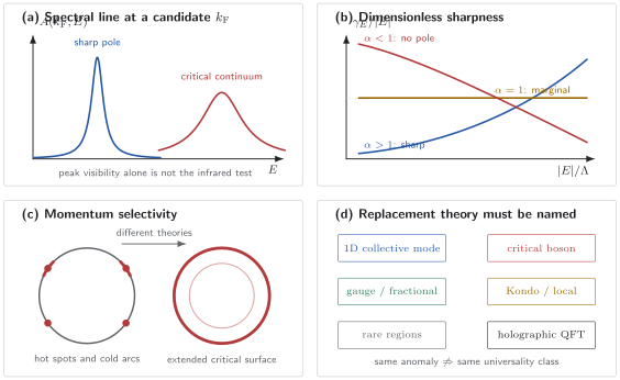
Non-Fermi-liquid diagnosis is multi-axis. A visible peak need not become asymptotically sharp; a singular self-energy may affect hot spots or an extended Fermi surface; and similar spectra can arise from distinct infrared mechanisms. The limiting ratio $\gamma_E/\lvert E\rvert$, momentum resolution, and independent thermodynamic and transport tests must be read together.

Spectra: What to Measure

For a single electron,

$$A(\mathbf k,E) = -\frac{1}{\pi} \operatorname{Im}G^{\mathrm R}(\mathbf k,E).$$

Angle-resolved photoemission accesses the occupied part multiplied by matrix elements and the Fermi function; tunneling usually integrates over momentum with its own matrix-element weighting. A credible non-Fermi-liquid spectral analysis should therefore:

1. map the full momentum dependence rather than only one cut;
2. separate intrinsic linewidth from energy and momentum resolution;
3. enforce causality between real and imaginary self-energy components;
4. verify spectral-weight and sum-rule accounting;
5. test whether fitted exponents persist as temperature and energy decrease;
6. compare electron spectra with thermodynamic and two-particle probes.

An apparent absence of a peak can result from a matrix-element zero, band overlap, a gap, surface disorder, or insufficient resolution. Conversely, a finite-temperature peak can survive even when its width scales as fast as its energy and no asymptotic quasiparticle exists.

Quantum oscillations provide a complementary but subtle constraint. Oscillations imply coherent orbital quantization over a field- and temperature-dependent window. They can reveal an extremal momentum-space area and an effective cyclotron mass, but do not by themselves prove a zero-field Landau pole over the whole Fermi surface. Magnetic field can suppress competing order, change scattering, or create a distinct low-energy regime.

Transport Is Not a Self-Energy Meter

The dc conductivity is a current-correlation limit, not the inverse of a single-particle linewidth. In schematic notation,

$$\sigma_{xx}^{\mathrm{dc}} = \lim_{\omega\to0^+} \frac{1}{\omega} \operatorname{Im}\Pi_{J_xJ_x}^{\mathrm R}(\omega,\mathbf q=0),$$

with contact terms and conventions supplied by the Kubo Formula. The response contains current vertices, conservation laws, and momentum-relaxing processes. In a clean Galilean-invariant fluid, strong momentum-conserving electron–electron scattering need not produce finite dc resistivity at all.

Resistivity exponents are nonunique

A measured law

$$\rho(T) = \rho_0+A T^n$$

with $n\ne2$ is incompatible with the simplest isotropic Fermi-liquid transport model over that window. It is not a unique fingerprint of quasiparticle destruction. Phonons, disorder, Umklapp geometry, multiband conduction, hot and cold regions, fluctuating order, and crossover between rates can all change the fitted exponent.

If channels conduct in parallel,

$$\sigma_{xx} = \sum_a \sigma_{xx}^{(a)}, \qquad \rho_{xx} = \frac{1}{\sigma_{xx}},$$

so the longest-lived current-carrying sector can short-circuit a strongly scattered one. A singular hot-spot self-energy does not automatically determine the bulk resistivity.

A transport evidence ledger

Probe	Useful constraint	What it does not establish alone
dc resistivity	momentum-relaxation law and crossover scales	electron pole width or a unique dynamical exponent
optical conductivity	frequency-dependent weight, Drude coherence, and scaling	one relaxation rate without mass, vertex, and interband choices
thermal transport	entropy-carrying mobile channels	charge assignment without separating phonons and neutral modes
Hall and magnetotransport	carrier geometry, compensation, and field-dependent scattering	carrier density through a one-band formula in a correlated multiband metal
thermopower	particle–hole asymmetry and entropy per transported charge	a direct quasiparticle residue
Wiedemann–Franz test	relation between low-$T$ charge and heat transport	fractionalization from a finite-$T$ deviation alone

Transport becomes compelling when its crossover scales, anisotropy, field dependence, and spectral redistribution agree with a mechanism that also explains single-particle and thermodynamic data.

Candidate Infrared Mechanisms

One-dimensional collective fixed points

Generic gapless interacting systems in one dimension flow to collective bosonic theories. Fermion insertion creates many density waves, the momentum-distribution jump disappears, and spectral functions develop power-law thresholds. This is a controlled replacement of Landau theory, not merely a badly broadened Fermi liquid. The full construction belongs to Luttinger Liquid Preview.

A Fermi surface coupled to a critical boson

Near a metallic ordering transition, low-energy fermions and an order-parameter field must be treated together. A two-patch action has the schematic form

$$\begin{aligned} S={}& \int_k \psi_s^\dagger(k) \left( -i\omega+s v_{\mathrm F}k_\perp +\kappa k_\parallel^2 \right) \psi_s(k) \\ &+ \frac12\int_q D_0^{-1}(q)\lvert\phi(q)\rvert^2 +g\int_{k,q} \phi(q)\psi_s^\dagger(k+q)\psi_s(k). \end{aligned}$$

The Fermi surface Landau-damps the boson, while the boson generates a singular fermion self-energy. For a common two-dimensional nematic or transverse-gauge scaling structure, the Matsubara forms are

$$D^{-1}(\mathbf q,i\Omega_n) \sim q_\parallel^2 +\gamma\frac{\lvert\Omega_n\rvert}{\lvert q_\parallel\rvert}, \qquad \Sigma(i\omega_n) \sim -i\,\operatorname{sgn}(\omega_n) \lvert\omega_n\rvert^{2/3},$$

up to coefficients, analytic terms, and corrections that depend on the model and control scheme. After causal continuation, $-\operatorname{Im}\Sigma^{\mathrm R}(E)\propto\lvert E\rvert^{2/3}$. For a finite-wavevector spin-density-wave transition, only hot spots connected by the ordering vector are directly singular at leading order. For a zero-momentum nematic mode, an extended Fermi surface can be affected.

These theories are active research subjects. Large-$N$, dimensional, codimensional, and dynamical-exponent expansions each control selected quantities, but extrapolating to a physical two-dimensional metal can be subtle. Pairing and other instabilities may intervene.

Emergent gauge fields and fractionalization

A neutral spinon Fermi surface coupled to a gapless U(1) gauge field has the same patch-level tension: gapless fermions damp the gauge field, and gauge fluctuations destroy ordinary spinon quasiparticles. The physical electron may be gapped because charge is localized, so electron photoemission and neutral thermal response probe different operators.

More generally, fractionalization can produce an orthogonal metal whose electrical conductivity and thermodynamics resemble those of a Fermi liquid while the physical-electron spectral function is gapped. This is a sharp warning against defining a Fermi liquid from transport and heat capacity alone.

Kondo destruction and multichannel screening

An exactly overscreened multichannel Kondo impurity flows to a non-Fermi-liquid boundary fixed point. In a lattice, however, impurity exponents cannot simply be copied: coherence, intersite exchange, symmetry breaking, disorder, and Fermi-surface reconstruction enter. At some heavy-fermion critical points, collapse of Kondo entanglement is proposed to destroy quasiparticles across an extended Fermi surface. Kondo Lattices and Quantum Criticality give the required lattice and material evidence ledgers.

Local criticality and SYK-like models

The large-$N$ SYK family gives a controlled strongly interacting Green function without a quasiparticle pole. In its conformal regime,

$$G(\tau) \propto \frac{\operatorname{sgn}(\tau)} {\lvert\tau\rvert^{2\Delta}},$$

with $\Delta$ fixed by the interaction order. The baseline model has no spatial momentum, so it is not by itself a theory of electrical resistivity or a material Fermi surface. Transport appears only after specifying coupled dots, lattice structure, conserved charge, and momentum relaxation.

Disorder and rare regions

Broad distributions of local Kondo or coherence scales can generate power-law thermodynamics and anomalous transport. For example, a low-scale distribution

$$P(T_0) \propto T_0^{\lambda-1}, \qquad 0<\lambda<1,$$

makes rare regions with very small $T_0$ dominate low-temperature averages. This can mimic clean quantum-critical exponents while producing strong sample dependence, spatial inhomogeneity, and broad local-relaxation distributions. The disorder ensemble and typical-versus-average distinction must be measured, not treated as a nuisance parameter.

Mechanism	Where Landau theory fails	Controlled anchor	Central caveat
Luttinger liquid	electron pole becomes power-law thresholds	low-energy bosonization and exact one-dimensional models	dimensional crossover can restore quasiparticles
critical order parameter	hot spots or an extended Fermi surface acquire singular self-energy	patch theories and selected expansions	physical two-dimensional fixed point may be preempted
gauge-coupled Fermi surface	emergent fermion couples to a singular transverse gauge mode	special large-$N$ or exponent expansions	gauge-charged partons are not directly measured electrons
orthogonal metal	physical-electron spectrum is gapped while charge transport remains metallic	explicit fractionalized constructions	experimental operator matching is essential
Kondo destruction	Kondo coherence and Fermi-volume organization collapse	impurity fixed points and selected lattice approaches	lattice universality and material identification remain active
SYK-like local criticality	conformal continuum replaces a pole	disorder-averaged large-$N$ saddle	no momentum or conductivity without an added spatial model
electronic Griffiths regime	rare low-energy regions dominate averages	explicit disordered models	inhomogeneity can masquerade as clean scaling
holographic finite-density theory	composite-operator correlator has a non-Landau singularity	classical gravity in a specified large-$N$, strong-coupling limit	model-to-material map is not automatic

Relation to Quantum Field Theory

A Fermi surface is an unusual field-theory object because low-energy modes live near a codimension-one manifold rather than near a finite set of momenta. Renormalization rescales energy and momentum normal to each patch while leaving the Fermi-surface label as a continuous index. Couplings that look irrelevant by naive point-particle counting can remain important because there are infinitely many low-energy patches.

The patch action above is therefore a quantum field theory, but not usually a relativistic one. It has anisotropic scaling, Landau damping, a finite density, and a preferred frame. Ward identities still tie self-energies to conserved-current vertices, while the Fermi surface supplies nonlocal response and a large phase space of gapless particle–hole states. Why Many-Body QM Leads to QFT gives the broader bridge, and Renormalization Group Preview owns the general fixed-point language.

What holography computes

Gauge/gravity duality supplies nonperturbative correlators for selected large-$N$, strongly coupled quantum field theories at finite density. In early holographic finite-density constructions, a fermionic operator near a momentum $k_{\mathrm F}$ has a Green function of the schematic form

$$G^{\mathrm R}(k_\perp,E) \simeq \frac{h_1} {k_\perp-E/v_{\mathrm F}-h_2e^{i\theta}E^{2\nu}},$$

where the infrared exponent $\nu$ is set by the operator’s effective scaling dimension in the near-horizon sector. For $\nu<1/2$, the nonanalytic term dominates the linear-frequency term and the excitation is not Landau-like. At $\nu=1/2$, logarithms produce marginal behavior. This realizes a calculable family of critical Fermi-surface correlators.

What it does not establish is equally important. A holographic Green function is an exact or controlled result only for its declared boundary theory and gravity limit. Similarity to a material spectrum does not identify the material’s microscopic degrees of freedom, momentum-relaxation mechanism, finite-$N$ corrections, or unique dual geometry. Holography is a laboratory for possible strongly coupled infrared structures, not evidence by itself that a particular crystal has a gravity dual.

Evidence Matrix

A persuasive diagnosis joins observables that interrogate different structures.

Question	Primary evidence	Required cross-check
Is there a momentum-space singular surface?	momentum-resolved spectra or oscillatory probes	distinguish poles, zeros, reconstruction, and field-induced states
Are electron excitations asymptotically sharp?	intrinsic $A(\mathbf k,E)$ linewidth and residue scaling	resolution, Kramers–Kronig consistency, and sum rules
Is the anomaly momentum selective?	full Fermi-surface spectroscopy and anisotropic response	compare hot and cold regions under the same conditions
Is the regime a ground-state property?	decreasing-$T$ trajectory and vanishing crossover scales	exclude hidden order, pairing, localization, and heating
Which degrees of freedom carry entropy?	heat capacity, thermal transport, and susceptibility	subtract phonons, nuclei, and other neutral channels
How is current relaxed?	dc, optical, Hall, and geometry dependence	identify disorder, Umklapp, lattice, and vertex effects
Is the mechanism clean or disorder-driven?	local-probe distributions and sample dependence	compare typical and averaged observables

The best case is overconstrained: one mechanism predicts the location and dimensionality of singular momenta, the scaling of spectra, thermodynamics, and at least one two-particle response, while surviving changes in sample quality and fitting window.

Practical Inference Workflow

1. State the limiting claim. Distinguish a phase, a critical trajectory, and a finite-window regime.
2. Map the phase diagram. Identify order, pairing, localization, and dimensional-crossover scales before fitting exponents.
3. Locate the relevant momentum structure. Decide whether the whole Fermi surface, hot spots, pockets, or no momentum-resolved surface is implicated.
4. Audit the electron spectrum. Fit causal line shapes, deconvolve resolution, and track both width and weight.
5. Test dimensionless sharpness. Plot $\gamma_E/\lvert E\rvert$ or the corresponding finite-$T$ ratio rather than linewidth alone.
6. Separate operators. Identify whether each probe couples to electrons, spinons, order-parameter modes, local moments, or composite operators.
7. Reconstruct current relaxation. Include vertices, momentum conservation, Umklapp, disorder, and parallel channels.
8. Compare independent scales. Ask whether spectral, thermodynamic, optical, Hall, and crossover scales track one another.
9. Test alternatives. Vary disorder, field, pressure, strain, carrier density, frequency, and sample geometry where possible.
10. Report control and uncertainty. State which theoretical limit is controlled and which extrapolation to the material remains conjectural.

Common Mistakes

Calling every bad metal a non-Fermi liquid

Large resistivity or a short mean free path can occur at temperatures above a small coherence scale. The term should identify a failed low-energy organizing principle, not merely poor conductivity.

Equating a Fermi surface with a Fermi liquid

A singular momentum-space surface can survive without a Landau pole. Critical Fermi surfaces, fractionalized states, and holographic correlators make this distinction explicit.

Inferring transport directly from the self-energy

Single-particle decay and current relaxation have different angular weights and conservation constraints. A self-energy exponent is not automatically a resistivity exponent.

Treating linear resistivity as a universality class

Linear-$T$ resistivity appears in several mechanisms and crossover regimes. It must be paired with a tuning trajectory, optical weight accounting, and independent spectral or thermodynamic tests.

Ignoring cold regions

Hot spots can dominate spectroscopy while cold regions dominate conductivity. Momentum averaging can obscure both facts.

Calling every vanishing electron residue incoherent

The physical electron may fractionalize into other sharp or critical degrees of freedom. One must specify the operator and conserved quantum numbers carried by each excitation.

Extending a controlled limit without an error ledger

A large-$N$, small-$\epsilon$, impurity, infinite-dimensional, or classical-gravity solution is exact in a particular limit. Applying it to $N=2$ electrons in a two-dimensional lattice is a hypothesis that needs independent checks.

Forgetting preemption

Superconductivity, density-wave order, nematicity, or localization may terminate the scaling regime. Suppressing an order with field can also alter the state being diagnosed.

Exercises

1. Classify a power-law self-energy

Suppose at $T=0$

$$-\operatorname{Im}\Sigma^{\mathrm R}(E) = C\Lambda^{1-\alpha}\lvert E\rvert^\alpha, \qquad C>0.$$

For which values of $\alpha$ is the excitation asymptotically sharp if residue effects remain finite? Classify $\alpha=2$, $\alpha=1$, and $\alpha=2/3$.

Solution

The relevant ratio is

$$\frac{-\operatorname{Im}\Sigma^{\mathrm R}(E)}{\lvert E\rvert} = C\left( \frac{\lvert E\rvert}{\Lambda} \right)^{\alpha-1}.$$

It vanishes for $\alpha>1$, remains constant for $\alpha=1$, and diverges for $0<\alpha<1$. Thus $\alpha=2$ is asymptotically sharp, $\alpha=1$ is marginal, and $\alpha=2/3$ has no asymptotically sharp pole. If $Z(E)$ also vanishes, the full dressed width and residue must be analyzed together.

2. Residue in a marginal self-energy

For positive $E$ well below $E_c$, take

$$\operatorname{Re}\Sigma^{\mathrm R}(E) = -\lambda E\ln\!\left(\frac{E_c}{E}\right).$$

Find the scale-dependent derivative estimate for $Z(E)$ and determine its low-energy trend.

Solution

Differentiation gives

$$\frac{\partial\operatorname{Re}\Sigma^{\mathrm R}}{\partial E} = -\lambda \left[ \ln\!\left(\frac{E_c}{E}\right)-1 \right].$$

With the sign convention written in the question,

$$Z(E) \simeq \left[ 1+\lambda\ln\!\left(\frac{E_c}{E}\right)-\lambda \right]^{-1}.$$

The logarithm makes the derivative singular, so $Z(E)$ tends to zero slowly as $E\to0$. The formula is a scale-dependent pole estimate; sufficiently close to the singular point, the full causal Green function is more informative than a constant-residue expansion.

3. Cold-region short circuit

Two Fermi-surface sectors conduct in parallel. Let

$$\sigma_h(T)=\frac{a}{T}, \qquad \sigma_c(T)=\frac{b}{T^2}, \qquad a,b>0.$$

Find the leading low-$T$ resistivity. Does the linear scattering channel control it?

Solution

The total conductivity is

$$\sigma(T) = \frac{a}{T} + \frac{b}{T^2} = \frac{b+aT}{T^2}.$$

Therefore

$$\rho(T) = \frac{T^2}{b+aT} = \frac{T^2}{b} \left[ 1-\frac{a}{b}T+O(T^2) \right].$$

The longer-lived cold sector dominates the low-temperature conductivity, so the leading resistivity is quadratic even though the hot sector has a linear rate. Geometry, inter-sector scattering, and disorder can change this conclusion, which is why transport cannot be read from one hot-spot self-energy.

4. Why the marginal logarithm is required

Assume over a broad symmetric low-energy window that

$$\operatorname{Im}\Sigma^{\mathrm R}(E) \propto -\lvert E\rvert.$$

Use the Kramers–Kronig structure to explain why the real part cannot simply be proportional to $E$ with a constant coefficient.

Solution

The retarded real part is a principal-value transform,

$$\operatorname{Re}\Sigma^{\mathrm R}(E) = \frac{1}{\pi} \mathcal P \int dE' \frac{\operatorname{Im}\Sigma^{\mathrm R}(E')}{E'-E}.$$

For an even cusp $-\lvert E'\rvert$ cut off at $E_c$, subtracting the value at $E=0$ leaves an odd term proportional to

$$E\ln\!\left(\frac{E_c}{\lvert E\rvert}\right)$$

plus an analytic term proportional to $E$. The logarithm is therefore required by causality. Fitting the imaginary part to a linear cusp while using an unrelated constant-slope real part is internally inconsistent.

5. Phase or finite-window regime?

A material shows $\rho-\rho_0\propto T^{1.2}$ from $2$ to $20\,\mathrm K$ and a broad photoemission peak at $10\,\mathrm K$. Below $1.5\,\mathrm K$ it becomes superconducting. List four measurements or tuning tests needed before claiming a non-Fermi-liquid ground state.

Solution

Useful tests include: suppressing superconductivity with a tuning parameter while checking that the field or pressure does not create a different normal state; tracking the intrinsic linewidth-to-energy ratio toward lower $E$ and $T$; mapping momentum dependence to distinguish hot and cold regions; and locating any critical coupling through vanishing crossover scales on both sides. One should also test sample-quality dependence, optical spectral weight, thermodynamics, and competing order. The stated observations establish an anomalous finite window, not a ground-state non-Fermi liquid.

6. An orthogonal diagnostic

Two metallic phases have the same leading heat capacity, compressibility, and dc conductivity. In phase A, electron photoemission has a Fermi-surface pole. In phase B, the electron spectrum is gapped, but charge transport remains metallic. Can thermodynamics and dc transport alone distinguish the phases? What observation does?

Solution

No. By construction, those bulk observables agree at leading order. The phases differ in the operator that overlaps with the gapless charged fermion. Momentum-resolved electron addition or removal, tunneling, or another probe explicitly sensitive to the physical-electron spectral function distinguishes a pole in phase A from a gap in phase B. This is the defining lesson of an orthogonal metal: conventional-looking transport and thermodynamics do not guarantee an electron Landau quasiparticle.

Research Status and Open Problems

Several statements are well established: Landau quasiparticles have precise pole and sharpness criteria; one-dimensional Luttinger liquids provide controlled alternatives; multichannel Kondo impurities and large-$N$ SYK models have non-Fermi-liquid fixed points in declared limits; and finite-density holography can produce calculable non-Landau fermionic correlators.

The broad materials problem remains active. Central questions include:

• Which two-dimensional lattice Hamiltonians possess stable metallic non-Fermi-liquid ground states without being preempted by pairing or order?
• Which controlled expansions faithfully continue to the physical number of fermion flavors and dimensions?
• When does an entire Fermi surface become critical, and when do cold regions survive?
• How can experiments distinguish Kondo destruction, order-parameter criticality, fractionalization, disorder, and a low coherence scale when several fit the same transport exponent?
• Which transport bounds or “Planckian” parametrizations are invariant under choices of effective mass, spectral weight, and fitting model?
• What experimentally accessible observables most directly reveal emergent gauge charge or orthogonality between physical electrons and current-carrying fermions?
• Which lessons from SYK and holography survive finite $N$, spatial locality, lattice momentum, and realistic conservation laws?

Progress requires models and experiments to meet on the same multi-observable ledger rather than on one suggestive exponent.

Connections

• Fermi Liquid Theory Preview gives the baseline whose infrared criteria are tested here.
• Spectral Functions and Lifetime and Spectral Weight provide the exact pole, width, residue, continuum, and resolution conventions.
• Fractionalization distinguishes deconfined sectors from a merely broad electron spectrum and owns the spinon, holon, vison, and response-composition ledger.
• Emergent Gauge Fields derives the constrained gauge structure and transverse propagator underlying gauge-coupled spinon non-Fermi liquids.
• Quantum Criticality develops the material endpoint and crossover-fan inference problem.
• Heavy Fermions and Kondo Lattices apply the coherence, Fermi-volume, and Kondo-destruction diagnostics to $f$-electron materials.
• Disorder in Quantum Matter supplies the ensemble and sample-control ledger needed before invoking rare-region physics.
• Kubo Formula owns exact linear response and the order of transport limits.
• SYK Model Preview develops one controlled local non-Fermi-liquid model without importing spatial transport claims.

References

• L. D. Landau, “The theory of a Fermi liquid,” Soviet Physics JETP 3, 920–925 (1957). Foundational quasiparticle and energy-functional construction.
• F. D. M. Haldane, “Luttinger liquid theory of one-dimensional quantum fluids,” Journal of Physics C 14, 2585–2609 (1981). Harmonic-fluid fixed point and power-law one-dimensional correlations.
• C. M. Varma, P. B. Littlewood, S. Schmitt-Rink, E. Abrahams, and A. E. Ruckenstein, “Phenomenology of the normal state of Cu-O high-temperature superconductors,” Physical Review Letters 63, 1996–1999 (1989); erratum 64, 497 (1990). Marginal-Fermi-liquid phenomenology.
• I. Affleck and A. W. W. Ludwig, “Critical theory of overscreened Kondo fixed points,” Nuclear Physics B 360, 641–696 (1991). Boundary conformal-field-theory solution of multichannel Kondo non-Fermi-liquid fixed points.
• B. I. Halperin, P. A. Lee, and N. Read, “Theory of the half-filled Landau level,” Physical Review B 47, 7312–7343 (1993). Composite fermions coupled to an emergent gauge field.
• S. Sachdev and J. Ye, “Gapless spin-fluid ground state in a random quantum Heisenberg magnet,” Physical Review Letters 70, 3339–3342 (1993). Large-symmetry random-interaction ancestor of SYK-like local criticality.
• B. L. Altshuler, L. B. Ioffe, and A. J. Millis, “Low-energy properties of fermions with singular interactions,” Physical Review B 50, 14048–14064 (1994). Singular gauge interaction and nonanalytic fermionic response.
• O. Parcollet and A. Georges, “Non-Fermi-liquid regime of a doped Mott insulator,” Physical Review B 59, 5341–5360 (1999). Controlled large-degeneracy doped-Mott crossover with a low coherence scale.
• E. Miranda and V. Dobrosavljević, “Localization-induced Griffiths phase of disordered Anderson lattices,” Physical Review Letters 86, 264–267 (2001). Disorder-generated distributions of local scales and non-Fermi-liquid thermodynamics.
• V. Oganesyan, S. A. Kivelson, and E. Fradkin, “Quantum theory of a nematic Fermi fluid,” Physical Review B 64, 195109 (2001). Metallic nematic criticality and singular fermion dynamics.
• T. Senthil, “Critical Fermi surfaces and non-Fermi liquid metals,” Physical Review B 78, 035103 (2008). Scaling framework for a sharp Fermi surface without Landau quasiparticles.
• E. C. Andrade, E. Miranda, and V. Dobrosavljević, “Electronic Griffiths phase of the Mott transition,” Physical Review Letters 102, 206403 (2009). Spatially resolved rare-region mechanism near a disordered Mott transition.
• S.-S. Lee, “Low-energy effective theory of Fermi surface coupled with U(1) gauge field in 2+1 dimensions,” Physical Review B 80, 165102 (2009). Patch theory and large-$N$ difficulties for gauge-coupled fermions.
• M. A. Metlitski and S. Sachdev, “Quantum phase transitions of metals in two spatial dimensions. I. Ising-nematic order,” Physical Review B 82, 075127 (2010). Patch field theory for a critical Fermi surface coupled to nematic order.
• D. F. Mross, J. McGreevy, H. Liu, and T. Senthil, “Controlled expansion for certain non-Fermi-liquid metals,” Physical Review B 82, 045121 (2010). Combined expansion for gauge-field and nematic non-Fermi liquids.
• H. Liu, J. McGreevy, and D. Vegh, “Non-Fermi liquids from holography,” Physical Review D 83, 065029 (2011). Finite-density holographic fermion spectra and critical Fermi surfaces.
• T. Faulkner, H. Liu, J. McGreevy, and D. Vegh, “Emergent quantum criticality, Fermi surfaces, and AdS$_2$,” Physical Review D 83, 125002 (2011). Near-horizon scaling dimensions and the low-energy Green-function classification.
• R. Nandkishore, M. A. Metlitski, and T. Senthil, “Orthogonal metals: The simplest non-Fermi liquids,” Physical Review B 86, 045128 (2012). Fractionalized metal with conventional thermodynamics and transport but a gapped electron spectrum.
• M. A. Metlitski, D. F. Mross, S. Sachdev, and T. Senthil, “Cooper pairing in non-Fermi liquids,” Physical Review B 91, 115111 (2015). Pairing instabilities of critical and gauge-coupled Fermi surfaces.
• J. Maldacena and D. Stanford, “Remarks on the Sachdev–Ye–Kitaev model,” Physical Review D 94, 106002 (2016). Large-$N$ conformal dynamics and four-point functions in SYK.

Summary

A non-Fermi liquid is established by the failure of Landau’s low-energy quasiparticle organization, not by one unusual exponent. The core spectral tests are residue, analytic structure, and the limiting width-to-energy ratio, resolved across momentum. Transport adds independent information only after current vertices and momentum relaxation are identified. One-dimensional collective modes, critical bosons, emergent gauge fields, Kondo destruction, SYK-like local criticality, rare regions, and holographic theories supply distinct replacement mechanisms with distinct control parameters. A mature claim states whether it concerns a phase, a critical trajectory, or a finite window, then makes spectra, thermodynamics, transport, tuning, and disorder agree on the same infrared account.