Lifetime and Spectral Weight

A quasiparticle is useful only within a validity window. It must remain identifiable long enough, propagate far enough, and carry enough weight in an appropriate operator channel for particle-like predictions to be controlled.

Three quantities are central:

$$\begin{gathered} E_{\mathbf k}^\star \quad \text{peak or pole energy}, \\ \Gamma_E(\mathbf k) \quad \text{energy FWHM}, \\ Z_{\mathbf k} \quad \text{coherent pole weight}. \end{gathered}$$

None is sufficient alone. A high narrow peak can have tiny area. A finite residue can accompany a width comparable to the branch separation. A long population lifetime can coexist with rapid phase dephasing. A transport lifetime can be much longer than a single-particle lifetime.

The operational question is therefore not simply

$$\text{“Does a peak exist?”}$$

but

$$\begin{gathered} \text{Which analytic singularity} \\ \text{and operator channel} \\ \text{produce the feature?} \\ \text{Which decay or dephasing} \\ \text{scale sets its intrinsic width?} \\ \text{Which transport or resolution} \\ \text{scale sets its observed width?} \\ \text{Against which energy, time,} \\ \text{length, and branch scales is it narrow?} \end{gathered}$$

This page develops that decision framework.

Scope and Canonical Ownership

This page owns the operational criteria for deciding when particle-like or mode-like language is reliable:

• the fixed dictionary among a complex pole, Lorentzian HWHM, FWHM, population lifetime, and quality factor;
• how a self-energy produces energy renormalization, residue, and intrinsic width;
• decay rates from matrix elements, conservation laws, phase space, and occupation factors;
• the distinction among single-particle, transport, phase-coherence, energy-relaxation, and collective-mode lifetimes;
• residue and coherent spectral weight as operator-dependent overlaps;
• pole-weight transfer among branches and continua;
• dimensionless narrowness, branch-separation, propagation, and Ioffe–Regel-type tests;
• how broad continua, threshold singularities, and nonexponential time dependence limit lifetime language;
• practical extraction and validation workflows for theory, numerics, and experiment.

Neighboring pages retain their canonical subjects:

• Spectral Functions owns the exact cross-channel dictionary for lines, poles, continua, line shapes, normalization, and measured-intensity forward models.
• Green Functions in Many-Body QM owns the full addition/removal Lehmann representation, Dyson equation, analytic continuation, and single-particle sum rules.
• Quasiparticles Overview owns the general emergent-particle concept, quantum numbers, effective Hamiltonian, and representative species.
• Time-Dependent Correlations owns dephasing, recurrence, threshold tails, finite-time windows, and Fourier duality in depth.
• Fermi’s Golden Rule owns the derivation and validity conditions of the long-time transition-rate formula.
• Diagrammatic Methods Preview owns self-energy diagrams, cutting logic, dressed propagators, and double-counting control.
• Transport Coefficients Preview owns conductivity, diffusion, current relaxation, hydrodynamic limits, and Drude-weight conventions.
• Analytic Continuation owns what imaginary-time data can and cannot identify about real-frequency widths.
• Sum Rules owns exact spectral moments and complete-weight accounting.

The formulas below are deliberately compact. Their purpose is to connect those canonical constructions into one quasiparticle-validity audit without duplicating their full derivations.

Convention Ledger

Energy variable

The spectral variable is energy,

$$E = \hbar\omega.$$

The page uses

$$A(\mathbf k,E) = - \frac1\pi \operatorname{Im} G^{\mathrm R}(\mathbf k,E)$$

for a diagonal single-particle spectral function. Its units are inverse energy.

Retarded sign

Write

$$\Sigma^{\mathrm R} = \Sigma' + i\Sigma''.$$

For a passive normal fermionic channel,

$$\Sigma''(\mathbf k,E) \le0.$$

Retarded poles lie on or below the real axis. A pole in the upper half-plane would represent exponential growth and signals an instability, a sign error, or a nonretarded convention.

Pole and width

A weakly damped pole is written

$$\mathcal E_{\mathbf k} = E_{\mathbf k}^\star - i\gamma_E(\mathbf k), \qquad \gamma_E>0.$$

The time-domain pole amplitude varies as

$$e^{-iE_{\mathbf k}^\star t/\hbar} e^{-\gamma_Et/\hbar}.$$

For the associated Lorentzian spectral peak:

$$\begin{aligned} \text{HWHM} &= \gamma_E, \\ \text{FWHM} &= \Gamma_E = 2\gamma_E. \end{aligned}$$

This page reserves $\Gamma_E$ for the energy FWHM.

Population lifetime

The pole amplitude decays with time constant

$$\tau_{\mathrm{amp}} = \frac{\hbar}{\gamma_E}.$$

Its squared magnitude decays as

$$e^{-2\gamma_Et/\hbar} = e^{-t/\tau_{\mathrm{pop}}},$$

so the population lifetime is

$$\tau_{\mathrm{pop}} = \frac{\hbar}{2\gamma_E} = \frac{\hbar}{\Gamma_E}.$$

Many authors call $\tau_{\mathrm{pop}}$ simply the quasiparticle lifetime. Others quote an amplitude decay time or use $\Gamma$ for the HWHM. A numerical linewidth–lifetime statement is meaningless until these choices are explicit.

Residue

For a canonical fermionic orbital,

$$\int_{-\infty}^{\infty} dE\, A(\mathbf k,E) =1.$$

If one coherent pole has area $Z_{\mathbf k}$, then

$$0\le Z_{\mathbf k}\le1$$

for that normalized diagonal channel. This bound does not carry unchanged to every bosonic response, matrix element, or experimentally weighted spectrum.

Four Complementary Tests

Spectral test

A peak should be narrow compared with the energy scale on which its center, background, matrix element, and self-energy vary:

$$\Gamma_E \ll \Delta_E^{\mathrm{local}}.$$

There is no universal choice of $\Delta_E^{\mathrm{local}}$. It may be a gap, excitation energy, neighboring-branch separation, distance to a threshold, or curvature scale.

Temporal test

The excitation should survive many characteristic oscillations:

$$\tau_{\mathrm{pop}} \gg \frac{\hbar} {\Delta_E^{\mathrm{dyn}}}.$$

For a mode with positive frequency $\Omega$ and damping rate $\gamma_t$ in inverse-time units, an equivalent quality factor is

$$\mathcal Q = \frac{\Omega}{2\gamma_t}.$$

The excitation is sharply underdamped when $\mathcal Q\gg1$.

Propagation test

For a wave packet with group velocity

$$\mathbf v_g = \frac1\hbar \nabla_{\mathbf k} E_{\mathbf k}^\star,$$

define

$$\ell_{\mathbf k} = \lvert\mathbf v_g\rvert \tau_{\mathrm{pop}}.$$

A propagating quasiparticle should travel many characteristic wavelengths or packet widths:

$$\ell_{\mathbf k} \gg \max \left( \frac{2\pi}{k}, w \right).$$

The rough crossover $k\ell\sim1$ is often called an Ioffe–Regel criterion. It is a diagnostic crossover, not a universal phase-transition theorem.

Identity and weight test

A branch label is useful only if the associated eigenvector or pole projector varies smoothly and remains distinguishable from nearby structures. Useful diagnostics include

$$Z_{\mathbf k}, \qquad \frac{\Gamma_E}{\Delta_{\mathrm{sep}}}, \qquad \langle O|\mathcal P_{\mathrm{pole}}|O\rangle.$$

Small $Z$ in one operator channel does not destroy the excitation. It says that this operator has little overlap with it. Loss of a useful particle description is stronger: width comparable to separation, rapid eigenvector exchange, vanishing weight in all simple channels, or no controlled pole expansion.

Pole Expansion from the Self-Energy

Dyson denominator

For one scalar channel,

$$G^{\mathrm R}(\mathbf k,E) = \frac1{ E-\xi_{\mathbf k} -\Sigma^{\mathrm R}(\mathbf k,E) }.$$

A candidate real quasiparticle energy satisfies

$$E_{\mathbf k}^\star - \xi_{\mathbf k} - \Sigma' \left( \mathbf k,E_{\mathbf k}^\star \right) =0.$$

This real-axis equation is only a starting point. It can have several roots, no isolated root, or a root in a region where $\Sigma''$ is too large for a quasiparticle expansion.

Residue from the real part

If the self-energy is smooth over the peak,

$$Z_{\mathbf k} = \left[ 1- \left. \partial_E \Sigma'(\mathbf k,E) \right|_{E=E_{\mathbf k}^\star} \right]^{-1}.$$

The derivative measures how strongly the medium’s dynamical response follows a shift of the excitation energy. Through causality, this real-part renormalization is linked to the frequency dependence of $\Sigma''$; mass renormalization and decay are not unrelated fitting knobs.

Width from the imaginary part

To leading order in weak damping,

$$\gamma_E(\mathbf k) = - Z_{\mathbf k} \Sigma'' \left( \mathbf k,E_{\mathbf k}^\star \right).$$

Therefore

$$\Gamma_E(\mathbf k) = - 2Z_{\mathbf k} \Sigma'' \left( \mathbf k,E_{\mathbf k}^\star \right).$$

The population rate is

$$\frac1{\tau_{\mathrm{pop}}} = \frac{\Gamma_E}{\hbar} = - \frac{ 2Z_{\mathbf k} \Sigma''(\mathbf k,E_{\mathbf k}^\star) }{\hbar}.$$

Dropping $Z$ is justified only when the chosen on-shell approximation and self-energy convention make it consistent.

Coherent and incoherent pieces

Near an isolated pole,

$$\begin{aligned} G^{\mathrm R}(\mathbf k,E) \simeq{}& \frac{Z_{\mathbf k}}{ E-E_{\mathbf k}^\star +i\gamma_E } \\ &+ G_{\mathrm{inc}}^{\mathrm R} (\mathbf k,E). \end{aligned}$$

The coherent spectral contribution is

$$A_{\mathrm{coh}}(\mathbf k,E) = \frac{Z_{\mathbf k}}{\pi} \frac{\gamma_E}{ \left( E-E_{\mathbf k}^\star \right)^2 +\gamma_E^2 }.$$

Its area is

$$\int dE\, A_{\mathrm{coh}} = Z_{\mathbf k},$$

while its peak height is

$$A_{\mathrm{coh}}^{\max} = \frac{Z_{\mathbf k}} {\pi\gamma_E}.$$

Height therefore mixes weight and width. A tall peak need not carry much spectral weight.

Matrix-valued channels

For orbitals, bands, Nambu components, or coupled modes,

$$\mathbf G^{\mathrm R} = \left[ E\mathbf1 - \mathbf H_0 - \boldsymbol\Sigma^{\mathrm R} \right]^{-1}.$$

The pole residue is a matrix or projector, not one scalar attached independently to every diagonal element. Near a simple non-Hermitian pole,

$$\mathbf G^{\mathrm R} \sim \frac{ |\psi_R\rangle \langle\psi_L| }{ \langle\psi_L| \partial_E\mathbf D |\psi_R\rangle } \frac1{E-\mathcal E_\star},$$

where

$$\mathbf D = E\mathbf1-\mathbf H_0-\boldsymbol\Sigma^{\mathrm R}.$$

Left and right eigenvectors differ when damping makes the effective problem non-Hermitian. Tracking only the largest diagonal peak can swap branch identity near a hybridization.

From Decay Matrix Elements to Widths

Exact eigenstates do not decay

An exact eigenstate of a closed, time-independent Hamiltonian evolves only by a phase. Decay language refers instead to

• a state prepared by a simple microscopic operator;
• a metastable resonance embedded in a continuum;
• an excitation of an effective Hamiltonian coupled to omitted degrees of freedom;
• a subsystem state after environmental degrees of freedom are traced out;
• a wave packet or mode amplitude whose overlap spreads among exact eigenstates.

This distinction prevents the phrase “the state decays” from hiding which projection or observable is losing weight.

Golden-rule benchmark

Let a weak interaction $V$ couple an initial prepared state $|i\rangle$ to a dense set of final states $|f\rangle$. In the long-time weak-coupling regime,

$$\frac1{\tau_i} = \frac{2\pi}{\hbar} \sum_f \left| \langle f|V|i\rangle \right|^2 \delta(E_f-E_i).$$

With the population-lifetime convention,

$$\Gamma_{E,i} = \frac{\hbar}{\tau_i} = 2\pi \sum_f \left| \langle f|V|i\rangle \right|^2 \delta(E_f-E_i).$$

The rate is not “matrix element squared” alone. It is the product of

$$\begin{aligned} &\text{coupling strength} \\ &\quad\times \text{available phase space} \\ &\quad\times \text{occupation factors} \\ &\quad\times \text{selection rules}. \end{aligned}$$

The delta function is an ideal long-time limit. At short time, strong coupling, a sharp threshold, or a sparse final spectrum, a constant Markovian rate need not emerge.

Conservation and symmetry

For a translationally invariant one-to-two decay,

$$a(\mathbf k) \longrightarrow b(\mathbf q) + c(\mathbf k-\mathbf q),$$

the energy constraint is

$$E_a(\mathbf k) = E_b(\mathbf q) + E_c(\mathbf k-\mathbf q).$$

On a lattice, momentum conservation permits a reciprocal vector:

$$\mathbf k = \mathbf q + \mathbf k' + \mathbf G.$$

Even when these equations have solutions, decay can be forbidden by spin, parity, point-group representation, charge, topological sector, or a vanishing matrix element.

A branch below the minimum allowed continuum,

$$E_a(\mathbf k) < E_{\mathrm{cont}}^{\min}(\mathbf k),$$

is kinematically stable against that channel at zero temperature.

Bose enhancement and Pauli blocking

For a bosonic decay channel, a schematic finite-temperature factor is

$$\left[ 1+n_B(E_b) \right] \left[ 1+n_B(E_c) \right].$$

Existing bosons stimulate final-state occupation. For fermionic final states, the corresponding availability factor is

$$\left[ 1-f(E_b) \right] \left[ 1-f(E_c) \right].$$

Occupied fermion states are Pauli blocked.

A full collision integral also contains inverse processes. For example, absorption of a thermal boson carries a factor $n_B$, while emission carries $1+n_B$. Equilibrium detailed balance makes the gain and loss terms cancel for the equilibrium distribution even though individual scattering events continue.

Imaginary self-energy and unitarity

The imaginary part of a retarded self-energy summarizes the probability flux from the projected one-particle channel into allowed intermediate and final states. Perturbatively, cutting rules and the optical theorem connect

$$-2\operatorname{Im}\Sigma^{\mathrm R}$$

to sums of on-shell transition probabilities.

The relation is structural, but factors of $Z$, $2$, $\hbar$, degeneracy, and normalization depend on whether one quotes

• an on-shell bare self-energy;
• a dressed pole width;
• an amplitude rate;
• a population rate;
• an energy HWHM or FWHM.

This page’s dressed population result is

$$\frac1{\tau_{\mathrm{pop}}} = - \frac{2Z}{\hbar} \operatorname{Im}\Sigma^{\mathrm R} (E^\star).$$

Threshold nonanalyticity

Suppose a continuum begins at $E_{\mathrm{th}}$ with weighted density

$$\rho_V(E) \propto \Theta(E-E_{\mathrm{th}}) \left( E-E_{\mathrm{th}} \right)^\alpha.$$

Golden-rule phase space then turns on nonanalytically at threshold. The real part of the self-energy develops a related cusp or singular derivative through dispersion relations.

Near the edge, treating $\Sigma'$ and $\Sigma''$ as constants across the peak can fail. Possible outcomes include

• a stable bound state below threshold;
• a narrow resonance above threshold;
• an asymmetric threshold enhancement;
• a virtual state;
• complete dissolution into continuum weight.

Common microscopic channels

Intrinsic many-body broadening can arise from

• quasiparticle–quasiparticle scattering;
• emission or absorption of phonons, magnons, photons, or other collective modes;
• decay of one collective quantum into two or more lower-energy quanta;
• Landau damping into particle–hole pairs;
• interband transitions;
• multipair production;
• Umklapp processes;
• coupling to a bath or lead retained in an open-system description.

Elastic disorder can broaden momentum-resolved single-particle spectra without transferring energy. Static inhomogeneity can broaden an ensemble spectrum without giving every microscopic realization the same decay rate.

Which Lifetime?

Single-particle spectral lifetime

The single-particle lifetime measures loss of overlap with a specified added- or removed-particle channel. In the pole regime,

$$\tau_{\mathrm{sp}} = \frac{\hbar}{\Gamma_E}.$$

Every process that scatters amplitude out of the chosen momentum, band, spin, and orbital channel can contribute.

Transport lifetime

Transport asks how quickly a current or another flux relaxes. For isotropic elastic scattering with angular probability $W(\theta)$,

$$\frac1{\tau_{\mathrm{sp}}} \propto \int d\Omega\, W(\theta),$$

whereas

$$\frac1{\tau_{\mathrm{tr}}} \propto \int d\Omega\, W(\theta) \left( 1-\cos\theta \right).$$

Small-angle scattering changes momentum only slightly. It can strongly broaden a momentum-resolved spectral peak while relaxing electrical current inefficiently:

$$\tau_{\mathrm{tr}} \gg \tau_{\mathrm{sp}}$$

is therefore possible.

Population and phase coherence

For a two-level coherence in a simple Markovian benchmark,

$$\frac1{T_2} = \frac1{2T_1} + \frac1{T_\phi}.$$

Here $T_1$ is a population-relaxation time and $T_\phi$ is pure dephasing. The coherence time $T_2$ can be shorter than the population lifetime even when no extra population decay occurs.

A single-particle Green function, a density response, and an off-diagonal coherence probe different operators. Their widths need not yield the same $T_1$ or $T_2$.

Energy-relaxation lifetime

Elastic scattering can destroy momentum or phase coherence while leaving energy unchanged. Energy relaxation weights processes by transferred energy and may require multiple collisions.

Thus

$$\tau_{\mathrm{energy}}, \qquad \tau_{\mathrm{tr}}, \qquad \tau_{\mathrm{sp}}$$

are distinct kinetic moments of a collision process.

Collective-mode attenuation time

For a collective pole

$$\omega_\star(\mathbf q) = \Omega(\mathbf q) - i\gamma_t(\mathbf q),$$

the mode amplitude decays as

$$e^{-\gamma_tt}.$$

Its amplitude decay time is $\gamma_t^{-1}$, while its quadratic energy or intensity decays on $(2\gamma_t)^{-1}$ in the ideal exponential model.

In a propagating mode with group velocity $v_g$, the temporal attenuation length is

$$\ell_{\mathrm{att}} = \frac{v_g}{\gamma_t}.$$

Experiments may instead fix real frequency and measure a complex wave vector

$$q_\star = q' + iq''.$$

Then amplitude decays spatially as $e^{-q''x}$. Converting between $q''$ and $\gamma_t$ requires the local dispersion and weak-damping approximation.

Escape and dwell time

In a finite device or open cavity, a linewidth can reflect escape into leads or radiation channels:

$$\Gamma_{\mathrm{tot}} = \Gamma_{\mathrm{int}} + \Gamma_{\mathrm{escape}}$$

when independent Markovian channels add at the level of rates. The escape width is physical but is not an intrinsic lifetime of the isolated material.

Lifetime dictionary

Quantity	What is lost?	Typical weighting
spectral lifetime	overlap with one operator-resolved excitation	all scattering out of the channel
transport lifetime	current or flux	angular or vertex weight
population lifetime	occupation of a prepared level or mode	gain–loss kinetics
coherence time	relative phase	population loss plus pure dephasing
energy-relaxation time	excess energy	transferred-energy weight
attenuation length	propagating amplitude in space	complex wave vector
escape time	probability inside a finite region	boundary coupling

Calling all of these “the scattering time” erases the observable being predicted.

Spectral Weight and Residue

Lehmann overlap

At zero temperature, an addition spectrum for a canonical fermion contains

$$\begin{aligned} A^+(\mathbf k,E) ={}& \sum_m \left| \langle \Psi_m^{N+1} | c_{\mathbf k}^\dagger | \Psi_0^N \rangle \right|^2 \\ &\times \delta \left( E- E_m^{N+1} + E_0^N + \mu \right), \end{aligned}$$

in one declared grand-canonical energy convention.

If one exact state or narrow resonance carries a coherent contribution, its residue is the corresponding operator overlap:

$$Z_{\mathbf k} = \left| \langle \Psi_{\mathrm{qp}}^{N+1} | c_{\mathbf k}^\dagger | \Psi_0^N \rangle \right|^2.$$

Residue is not a probability that an immortal bare particle sits inside the dressed excitation. It is the squared projection of one operator-prepared state onto one exact or resonant branch.

Operator dependence

Let two operators create different linear combinations of the same exact states:

$$\begin{aligned} O_1^\dagger|0\rangle &= a|\Phi\rangle + b|\Phi_\perp\rangle, \\ O_2^\dagger|0\rangle &= c|\Phi\rangle + d|\Phi_\perp\rangle. \end{aligned}$$

The same excitation $|\Phi\rangle$ has weights

$$Z_1 = |a|^2, \qquad Z_2 = |c|^2.$$

It can be bright in one channel and dark in another without changing its existence or energy.

Coherent versus incoherent weight

For a normalized diagonal canonical-fermion spectrum,

$$1 = Z_{\mathbf k} + \int dE\, A_{\mathrm{inc}}(\mathbf k,E)$$

when one coherent pole is isolated and all other weight is grouped as incoherent.

The incoherent part is not experimental noise. It can contain

• shake-up satellites;
• multiparticle continua;
• molecular or atomic branches;
• phonon sidebands;
• Hubbard bands;
• threshold singularities;
• additional coherent poles not selected into $Z$.

Calling everything outside the main peak “background” can discard most of the many-body physics.

Peak height is not weight

For a Lorentzian with fixed area $Z$,

$$A_{\max} = \frac{2Z}{\pi\Gamma_E}.$$

Narrowing the peak doubles its height when the FWHM is halved, even though the residue is unchanged. Conversely, a broad feature can carry substantial integrated weight while having a low maximum.

Experimental intensity adds matrix elements and occupation factors:

$$I(\mathbf k,E) \sim |M(\mathbf k,E)|^2 f(E) A(\mathbf k,E) \ast R.$$

The resolution kernel $R$ and probe matrix element $M$ must be removed or modeled before an intensity area can be called a quasiparticle residue.

Weight transfer under hybridization

Consider two lossless levels coupled by

$$\mathbf H = \begin{pmatrix} E_1 & g \\ g & E_2 \end{pmatrix}.$$

Define

$$\tan2\theta = \frac{2g}{E_1-E_2}.$$

If the probe creates only bare state $|1\rangle$, its weights in the two exact eigenmodes are

$$Z_+ = \cos^2\theta, \qquad Z_- = \sin^2\theta.$$

Their sum is conserved:

$$Z_++Z_-=1.$$

Across the avoided crossing, the peaks exchange weight smoothly. Following only the brighter peak can produce an apparent jump between eigenbranches.

Fermi-surface discontinuity

In a conventional Fermi liquid at zero temperature, the jump in momentum occupation at the Fermi surface equals the quasiparticle residue:

$$\lim_{\delta k\to0^+} \left[ n(k_F-\delta k) - n(k_F+\delta k) \right] = Z_{k_F}.$$

This is a special relation tied to the single-particle Green function and Fermi-liquid structure. It is not a universal definition of residue in every phase.

Bosonic and collective residues

For bosonic Nambu Green functions, residues can involve $u_{\mathbf k}^2$, $-v_{\mathbf k}^2$, and an indefinite metric. For a density or spin response, a pole coefficient has units set by the chosen operators and normalization.

Therefore statements such as

$$0\le Z\le1$$

must be restricted to a normalized positive diagonal channel. A collective-mode oscillator strength, a dielectric pole residue, and a fermionic addition probability are not the same quantity merely because all are called spectral weight.

Sum rules and partial windows

An exact sum rule constrains the complete spectrum:

$$m_n = \int dE\, E^nA(E).$$

A finite experimental window measures only

$$m_n^{[E_1,E_2]} = \int_{E_1}^{E_2} dE\, E^nA(E).$$

Missing high-energy satellites or negative-energy weight can make an apparent residue change even when the complete sum rule is satisfied. Track both the pole area and the closure of the relevant total moment.

Broad Continua and Non-Lorentzian Response

Continuum does not mean noise

In the thermodynamic limit, multiparticle energies can become dense. The analytic Green function then develops a branch cut rather than isolated poles. Its spectral weight can be smooth, singular at a threshold, or divided among several overlapping continua.

A continuum can represent perfectly coherent exact eigenstates of the full closed Hamiltonian. The apparent decay of a simple prepared state comes from dephasing among those many frequencies.

Survival amplitude

For a normalized spectral measure $\rho(E)$ associated with a prepared state,

$$\mathcal A(t) = \int dE\, \rho(E) e^{-iEt/\hbar}.$$

A pole approximation

$$\rho_{\mathrm{pole}}(E) = \frac1\pi \frac{\gamma_E}{ (E-E^\star)^2+\gamma_E^2 }$$

gives

$$\mathcal A_{\mathrm{pole}}(t>0) = e^{-iE^\star t/\hbar} e^{-\gamma_Et/\hbar}.$$

This exact exponential uses an ideal Lorentzian extending over the whole real axis. A physical Hamiltonian bounded below cannot preserve that form at arbitrarily short and long times.

Threshold tails

If

$$\rho(E) \sim \Theta(E-E_{\mathrm{th}}) \left( E-E_{\mathrm{th}} \right)^\alpha$$

with $\alpha>-1$, then the threshold contribution has long-time scaling

$$\mathcal A_{\mathrm{th}}(t) \propto e^{-iE_{\mathrm{th}}t/\hbar} t^{-(\alpha+1)}$$

up to a complex coefficient and powers of $\hbar$.

The late-time decay is a power law, not an exponential. Assigning one constant lifetime to a threshold-dominated spectrum loses the physically important exponent.

Short-time behavior

For a state with finite energy variance,

$$P(t) = \left| \mathcal A(t) \right|^2 = 1- \frac{(\Delta E)^2t^2}{\hbar^2} +O(t^3).$$

The survival probability begins quadratically, whereas a pure exponential begins linearly. Golden-rule exponential decay is therefore an intermediate-time approximation, not an exact identity at $t=0$.

Fano interference

When a probe reaches the same final continuum through a direct path and through a resonant discrete state, the amplitudes interfere. A standard reduced line shape is

$$I(\varepsilon) \propto \frac{ (q_F+\varepsilon)^2 }{ 1+\varepsilon^2 },$$

where

$$\varepsilon = \frac{2(E-E_r)}{\Gamma_E}.$$

The result can be an asymmetric peak, a peak–dip structure, or a near-zero. Its maximum and apparent half-width do not obey the elementary isolated-Lorentzian dictionary.

Inhomogeneous and instrumental broadening

If each microscopic region has a narrow Lorentzian but their center energies have a Gaussian distribution, the ensemble line is a Voigt profile. Its width contains both homogeneous and inhomogeneous contributions.

Similarly, a finite observation window convolves the intrinsic spectrum with a sinc-like or chosen window transform. A numerical regulator

$$\eta>0$$

replaces exact delta functions by plotting kernels. Neither operation creates an intrinsic many-body decay rate.

Finite systems

A finite closed system has discrete exact lines. Apparent smoothness can result when

$$\eta \gtrsim \Delta_{\mathrm{level}}$$

or when the observation time is too short to resolve the level spacing. A physical continuum requires a declared limit, reservoir, average, or experimental resolution.

The limits

$$L\to\infty, \qquad t_{\max}\to\infty, \qquad \eta\to0^+$$

need not commute.

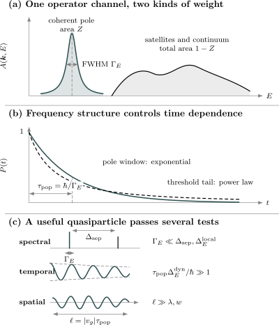
Three layers of the quasiparticle test. A pole of area $Z$ and FWHM $\Gamma_E$ can coexist with substantial incoherent weight. Its intermediate-time population decays as $e^{-t/\tau_{\mathrm{pop}}}$ with $\tau_{\mathrm{pop}}=\hbar/\Gamma_E$, while continuum thresholds produce nonexponential tails. Particle-like language is controlled only when width, propagation length, and branch separation are simultaneously favorable.

When Is the Excitation Well Defined?

Finite-energy narrowness

For a gapped or finite-energy branch measured relative to a physically relevant reference,

$$r_E := \frac{\Gamma_E}{ \lvert E^\star-E_{\mathrm{ref}} \rvert }.$$

The pole is parametrically sharp when

$$r_E\ll1.$$

The reference must be stated. For a particle excitation it may be the chemical potential; for a resonance it may be a threshold; for an optical mode it may be zero energy.

Gapless scaling

For a gapless branch, both energy and width can vanish:

$$E^\star(q)\to0, \qquad \Gamma_E(q)\to0.$$

The decisive ratio is

$$\frac{\Gamma_E(q)} {E^\star(q)}.$$

If it tends to zero, the branch becomes asymptotically sharp. If it approaches a nonzero constant, the mode has only a finite quality factor. If it diverges, the would-be excitation is overdamped in the infrared.

Quoting only $\Gamma_E\to0$ is insufficient: every low-energy scale may be vanishing at the same time.

Branch separation

Let

$$\Delta_{\mathrm{sep}}(\mathbf k) = \min_{\beta\ne\alpha} \left| E_\alpha(\mathbf k) - E_\beta(\mathbf k) \right|.$$

A scalar branch assignment requires

$$\Gamma_{E,\alpha} \ll \Delta_{\mathrm{sep}}.$$

Near an avoided crossing or exceptional point, use the full matrix response. A fit to independent Lorentzians can fail even when two visible maxima remain.

Distance to continuum

Define

$$\Delta_{\mathrm{cont}} = E_{\mathrm{th}} - E^\star$$

for a branch below a continuum. If $\Delta_{\mathrm{cont}}>0$, the channel is closed at zero temperature. If the branch lies above threshold, the local separation no longer protects it and the imaginary self-energy must be evaluated.

Near

$$\lvert\Delta_{\mathrm{cont}}\rvert \lesssim \Gamma_E,$$

threshold curvature usually invalidates a constant-width Lorentzian.

Smooth-self-energy test

The pole expansion assumes the self-energy changes little across one width. Schematic requirements are

$$\gamma_E \left| \partial_E\Sigma'' \right| \ll \lvert\Sigma''\rvert$$

and

$$\gamma_E^2 \left| \partial_E^2\Sigma' \right| \ll1.$$

These are local diagnostics, not exact inequalities with universal constants. A divergent derivative, nearby pole, or threshold singularity demands a non-Lorentzian treatment.

Propagation and Ioffe–Regel test

For a nearly monochromatic packet,

$$k\ell = k \lvert v_g\rvert \tau_{\mathrm{pop}}.$$

The regime

$$k\ell\gg1$$

supports many oscillations over a mean free path. When $k\ell$ becomes order unity, momentum and trajectory cease to be sharply resolved in a semiclassical picture.

For a lattice excitation near a Brillouin-zone boundary, $k^{-1}$ is not always the relevant size. Compare $\ell$ with the packet width, lattice spacing, and local wavelength measured relative to the band extremum.

Residue is supporting evidence

There is no universal threshold such as

$$Z>\frac12$$

for quasiparticle existence. A sharp eigenmode can have small weight in one microscopic operator. Conversely, a broad maximum can carry large integrated weight without yielding a long-lived particle.

Residue becomes decisive when combined with other failures:

$$Z\to0, \qquad \frac{\Gamma_E}{\Delta_{\mathrm{sep}}} \not\ll1, \qquad k\ell\not\gg1.$$

Together these indicate that the chosen particle language is losing predictive compression.

Controlled-theory test

A narrow numerical peak is trustworthy only if its width is stable under

• frequency and momentum resolution;
• finite-size scaling;
• regulator removal;
• basis or bond-dimension enlargement;
• self-consistency and vertex choices;
• analytic-continuation priors;
• conservation-law and sum-rule checks.

An unresolved width is an upper bound or a resolution statement, not a measured lifetime.

Representative Regimes

Fermi-liquid quasiparticles

For a conventional three-dimensional Fermi liquid near its Fermi surface, phase-space restriction and Pauli blocking give the schematic low-energy rate

$$\frac1{\tau_{\mathrm{sp}}} \sim \frac{ \xi^2 + (\pi k_BT)^2 }{ \hbar E_F }$$

times an interaction-dependent dimensionless coefficient. Here

$$\xi = E-\mu.$$

At zero temperature,

$$\frac{\hbar/\tau_{\mathrm{sp}}} {\lvert\xi\rvert} \propto \frac{\lvert\xi\rvert}{E_F} \longrightarrow0.$$

The quasiparticle becomes asymptotically sharp even though its lifetime diverges only as the Fermi surface is approached. In two dimensions, logarithmic factors can modify the simple quadratic law.

The Fermi Liquid Theory Preview page owns the Landau construction, effective mass, interaction function, and thermodynamic relations.

Electron–phonon threshold

At zero temperature, an electron can emit a dispersionless phonon of energy $\hbar\Omega_0$ only if its initial energy and momentum permit a final electronic state plus that phonon:

$$\xi_{\mathbf k} = \xi_{\mathbf k-\mathbf q} + \hbar\Omega_0.$$

Below the emission threshold, that channel contributes no real decay in the ideal clean model, though virtual phonons still renormalize the real self-energy and residue. At finite temperature, absorption appears with Bose factor

$$n_B(\Omega_0).$$

Thus an energy kink, residue change, and linewidth onset are causally related signatures of the same coupling, not independent effects.

Weak Bose-gas phonons

In a weakly interacting three-dimensional Bose condensate at zero temperature, a long-wavelength Bogoliubov phonon can decay by the Beliaev process into two lower-energy phonons. In the asymptotic regime,

$$\gamma_t(q) \propto q^5, \qquad \Omega(q) \propto q.$$

Therefore

$$\frac{\gamma_t(q)}{\Omega(q)} \propto q^4 \longrightarrow0.$$

The mode becomes sharply defined in the infrared even though decay is kinematically allowed. Curvature, dimension, temperature, and interaction range can change the available phase space.

Magnons and crystal phonons

Anharmonic phonons and interacting magnons can decay when one branch overlaps a symmetry-allowed multiparticle continuum. Their widths depend on cubic or quartic vertices, occupation factors, crystal momentum conservation, and density of states.

The canonical species pages own those Hamiltonians:

• Phonons as Many-Body Excitations
• Magnons

A dispersion entering a continuum does not guarantee large damping if the matrix element vanishes. A branch outside a two-particle continuum can still decay through disorder, higher-particle channels, or coupling to another subsystem.

Plasmons

A long-wavelength three-dimensional plasmon can lie above the one-pair particle–hole continuum and avoid ideal one-pair Landau damping. At larger momentum it can enter that continuum, lose pole weight, and broaden.

Plasmons Preview owns the dielectric zero, loss function, dimensional scaling, and $f$-sum-rule analysis. The lesson here is diagnostic: frequency, FWHM, and pole weight must all be tracked through continuum entry.

Polarons

A polaron pole can remain sharp while its bare-particle residue becomes small because much of the state resides in its dressing cloud. Conversely, a repulsive polaron branch may retain visible residue while having a finite decay width into a lower branch and host excitations.

The pair

$$\left( Z_{\mathrm{pol}}, \Gamma_{E,\mathrm{pol}} \right)$$

contains independent information. Polarons Preview owns the mobile-impurity construction and branch taxonomy.

One-dimensional continua

In a generic interacting one-dimensional fermion system, an injected microscopic fermion can fractionalize into collective spin and charge excitations. The single-fermion spectral function may have threshold power laws but no finite-residue pole:

$$Z=0.$$

This is not merely a quasiparticle with a very short Lorentzian lifetime. The correct low-energy language is collective and critical. Luttinger Liquid Preview owns that construction.

Critical and strongly incoherent regimes

Near a quantum critical point, the only low-energy scale can be temperature or frequency itself. A response may obey scaling such as

$$\Gamma_E \sim k_BT$$

or

$$\Gamma_E \sim \lvert E\rvert$$

without a small narrowness ratio. A broad universal scaling function can be physically precise even when quasiparticle language is not.

The absence of a sharp pole is not absence of theory. Hydrodynamic variables, critical operators, kinetic distributions, or fractionalized degrees of freedom may provide the controlled description.

Temperature, Disorder, and Multiple Channels

Thermal broadening

Temperature opens absorption channels, changes Bose and Fermi occupation factors, and smears sharp occupation boundaries. The retarded self-energy itself can be temperature dependent:

$$\Sigma^{\mathrm R} = \Sigma^{\mathrm R}(\mathbf k,E;T).$$

Do not infer the intrinsic zero-temperature residue by fitting a temperature-broadened peak with a fixed background and fixed matrix element.

Elastic disorder

For static weak disorder in a simple Born approximation,

$$\frac1{\tau_{\mathrm{el}}} \propto n_{\mathrm{imp}} \sum_{\mathbf k'} \left| U_{\mathbf k\mathbf k'} \right|^2 \delta \left( \xi_{\mathbf k} - \xi_{\mathbf k'} \right).$$

Energy is conserved, but momentum-resolved overlap decays. The transport rate adds an angular current-relaxation factor.

Disorder averaging can restore translation invariance statistically while hiding localization, rare regions, or sample-to-sample variation. A disorder-averaged width is not automatically the lifetime of one realization.

Rate addition and its limits

Independent weak Markovian channels often motivate Matthiessen-type addition:

$$\frac1{\tau_{\mathrm{tot}}} \simeq \sum_a \frac1{\tau_a}.$$

This approximation can fail when channels interfere, share intermediate states, alter the spectrum self-consistently, or have strong energy dependence. Adding fitted FWHMs is especially unsafe for non-Lorentzian or inhomogeneous lines.

Vertex selectivity

Two probes can report different apparent widths because they couple to different momentum regions, orbitals, polarizations, or many-body channels. A probe-dependent intensity is

$$I_O(E) \propto \langle O^\dagger \delta(E-H+E_0) O\rangle,$$

not the density of all states at that energy.

Agreement in peak energy does not require agreement in linewidth or residue.

Extracting Width and Weight

Begin with a forward model

An observed spectrum should be modeled schematically as

$$I_{\mathrm{obs}} = \left[ M \times F_{\mathrm{occ}} \times S_{\mathrm{intrinsic}} + B \right] \ast R.$$

Here $M$ is a probe matrix element, $F_{\mathrm{occ}}$ an occupation or detailed-balance factor, $B$ a background, and $R$ the instrument response. The intrinsic spectrum may itself contain several poles and continua.

Deconvolution is often ill conditioned. It is safer to convolve a causal intrinsic model forward and fit the observed data than to divide noisy data by a resolution function.

Energy-distribution curves

At fixed momentum, an energy-distribution curve samples

$$I(E) \propto |M(E)|^2 f(E) A(\mathbf k,E)$$

before convolution and backgrounds. A Lorentzian energy width can estimate $\Gamma_E$ only when

• the self-energy is smooth across the line;
• nearby bands and satellites are resolved or modeled;
• the occupation cutoff is treated;
• matrix elements and background vary slowly;
• instrumental and inhomogeneous widths are separated.

Near a threshold or Fano interference, the fitted Lorentzian center and width can be biased even at high signal-to-noise ratio.

Momentum-distribution curves

At fixed energy, suppose the bare dispersion is locally linear:

$$\xi_{\mathbf k} \simeq v_0 \left( k-k_0 \right),$$

where $v_0$ has units of energy times length. If $\Sigma$ is nearly independent of momentum, the momentum-distribution curve is approximately Lorentzian with HWHM

$$\delta k \simeq \frac{ -\Sigma''(E) }{ \lvert v_0\rvert }.$$

Converting this to an energy FWHM by multiplying by a measured velocity requires care. Strong momentum dependence, band curvature, matrix-element variation, overlapping bands, and a momentum-dependent background invalidate the elementary relation.

Damped-oscillator modes

A common collective-response model is

$$\chi^{\mathrm R}(\omega) = \frac{ \chi_0\Omega_0^2 }{ \Omega_0^2 - \omega^2 - 2i\gamma_t\omega }.$$

Its poles are

$$\omega_\pm = \pm \sqrt{ \Omega_0^2-\gamma_t^2 } - i\gamma_t.$$

For $\gamma_t\ll\Omega_0$, the positive-frequency peak is locally Lorentzian with angular-frequency FWHM approximately

$$\Gamma_\omega \simeq 2\gamma_t.$$

When damping is not weak, the peak maximum, real part of the pole, and undamped parameter $\Omega_0$ differ appreciably. Quoting one of them as “the mode frequency” without the model is ambiguous.

Resolution and Voigt profiles

A Lorentzian intrinsic line convolved with a Gaussian resolution gives a Voigt profile. If their FWHMs are $\Gamma_L$ and $\Gamma_G$, a useful approximation is

$$\begin{aligned} \Gamma_V \simeq{}& 0.5346\,\Gamma_L \\ &+ \sqrt{ 0.2166\,\Gamma_L^2 + \Gamma_G^2 }. \end{aligned}$$

The observed FWHM is not the sum in quadrature of two arbitrary line shapes. Resolution parameters should be calibrated independently when possible.

Integrating weight

Define the weight of one resolved component over a declared window:

$$W_{\mathrm{peak}} = \int_{E_1}^{E_2} dE\, \left[ A(E)-A_{\mathrm{base}}(E) \right].$$

Systematic uncertainty in the baseline can dominate statistical fit uncertainty for broad peaks. Vary the window, baseline family, resolution, and number of components. Report how much of the exact or known sum rule lies outside the window.

Coupled peaks

If two modes hybridize, fit a matrix response or a coupled-mode denominator. Independent peak fits do not enforce

• common poles across channels;
• causal real and imaginary parts;
• oscillator-strength conservation;
• shared damping pathways;
• eigenvector continuity.

A physically constrained fit can require fewer meaningful parameters than several unrelated Lorentzians.

Computational Routes and Audits

Perturbative self-energies

At weak coupling, compute $\Sigma^{\mathrm R}(\mathbf k,E)$ and solve either

• an on-shell approximation using the reference energy;
• a quasiparticle equation for the real part;
• the full complex pole equation.

State which was used. Self-consistent dressing can improve some regimes and violate others if vertices are not updated consistently.

Kinetic equations

A Boltzmann or quantum kinetic equation resolves gain and loss rates for distribution functions. It is the natural tool for transport, energy relaxation, and nonequilibrium populations, but it may discard off-shell spectral structure and coherent memory. Boltzmann Transport gives the canonical material-level collision operator, relaxation-time reduction, transport lifetime, and electrical and thermal response.

The collision integral must preserve the intended conserved quantities:

$$\sum_{\mathbf k} \mathcal I_{\mathrm{coll}}[f] =0$$

for number-conserving scattering, with analogous weighted identities for energy and momentum where appropriate.

Exact diagonalization and Krylov spectra

Finite-size exact spectra are sums of delta functions. Introduced broadening $\eta$ is a visualization and resolution scale:

$$\delta(E-E_n) \longrightarrow \frac1\pi \frac{\eta}{ (E-E_n)^2+\eta^2 }.$$

Vary $\eta$ independently of system size. A stable physical width should not simply track the chosen regulator.

Real-time evolution

Real-time methods can extract decay envelopes directly, but finite duration limits energy resolution:

$$\Delta E \sim \frac{\hbar}{t_{\max}}.$$

Window choice changes spectral leakage and apparent FWHM. Entanglement growth, boundary reflections, and finite-size recurrences set additional time limits.

Fit exponential, stretched-exponential, Gaussian, and power-law forms only where the corresponding residuals and physical mechanisms support them.

Imaginary-time data

Imaginary-time correlators smooth real-frequency structure through an integral kernel. Several spectra with different narrow linewidths can agree within the same statistical errors.

A continued peak width is trustworthy only if synthetic-resolution tests, covariance, sum rules, positivity, prior variation, and alternative continuations show that the width is identifiable. Otherwise report a bound or resolution limit.

Causality and positivity

A normal diagonal fermionic spectrum must obey

$$A(\mathbf k,E)\ge0.$$

The retarded Green function must be analytic in the upper half-plane, and its real and imaginary parts must satisfy dispersion relations. Negative diagonal weight, an upper-half-plane pole, or a violated normalization is not a novel lifetime effect.

Conservation and vertex consistency

A self-energy approximation can generate a plausible single-particle width while an inconsistent response vertex violates a Ward identity or sum rule. When using the same approximation to infer transport or density-mode lifetimes, check the associated conserved-current constraints.

Reliable Workflow

1. Name the channel. State the operator, state, momentum label, and whether the spectrum adds a particle, removes one, or preserves number.
2. Fix units. Distinguish energy width $\Gamma_E$, angular-frequency width $\Gamma_\omega$, and inverse-time rate.
3. Declare HWHM or FWHM. Do not use $\Gamma$ before this choice.
4. Identify the analytic structure. Distinguish a real pole, complex resonance, threshold, branch cut, and overlapping modes.
5. Map decay channels. Enforce energy, momentum, charge, spin, symmetry, and occupation constraints.
6. Choose the comparison scale. Use excitation energy, branch separation, continuum distance, packet size, or a local dispersion scale.
7. Check pole smoothness. Inspect self-energy variation over one fitted width.
8. Separate lifetimes. Do not substitute transport, coherence, escape, or energy-relaxation times for a spectral lifetime.
9. Track integrated weight. Fit area and sum-rule fraction, not peak height alone.
10. Model the probe. Include matrix elements, occupations, backgrounds, final states, and resolution.
11. Scale numerical regulators. Vary size, time window, broadening, basis, and continuation assumptions independently.
12. Report a validity window. State the range of momentum, energy, temperature, and resolution where the quasiparticle interpretation is supported.

Worked Checks

Self-energy factors of two

Suppose a quasiparticle root occurs at

$$E^\star = 0.30\ {\mathrm{eV}},$$

with

$$\left. \partial_E\Sigma' \right|_{E^\star} = -1.5$$

and

$$\Sigma''(E^\star) = -25\ {\mathrm{meV}}.$$

The residue is

$$Z = \frac1{1-(-1.5)} = 0.4.$$

The dressed HWHM is

$$\gamma_E = -Z\Sigma'' = 10\ {\mathrm{meV}},$$

so

$$\Gamma_E = 20\ {\mathrm{meV}}.$$

Using

$$\hbar \simeq 658.2\ {\mathrm{meV\,fs}},$$

the population lifetime is

$$\tau_{\mathrm{pop}} = \frac{\hbar}{\Gamma_E} \simeq 32.9\ {\mathrm{fs}}.$$

Using $\hbar/\gamma_E$ would instead give the amplitude decay time, twice as long.

Equal residue, unequal height

Take two Lorentzians with the same area

$$Z=0.20$$

but HWHMs

$$\gamma_{E,1} = 5\ {\mathrm{meV}}, \qquad \gamma_{E,2} = 20\ {\mathrm{meV}}.$$

Their peak-height ratio is

$$\frac{A_1^{\max}} {A_2^{\max}} = \frac{\gamma_{E,2}} {\gamma_{E,1}} =4.$$

The first peak is four times taller, yet both carry the same coherent weight.

Forward scattering

Suppose elastic scattering is concentrated near a small angle $\theta_0\ll1$. Then

$$1-\cos\theta \simeq \frac{\theta^2}{2}.$$

If the angular distribution is narrow enough to replace $\theta^2$ by $\theta_0^2$, then

$$\frac1{\tau_{\mathrm{tr}}} \simeq \frac{\theta_0^2}{2} \frac1{\tau_{\mathrm{sp}}}.$$

For

$$\theta_0=0.10,$$

one estimates

$$\tau_{\mathrm{tr}} \simeq 200\,\tau_{\mathrm{sp}}.$$

A broad single-particle line can therefore coexist with relatively efficient current flow.

Fermi-liquid scale estimate

Use the schematic coefficient-one estimate

$$\Gamma_E \sim \frac{\xi^2}{E_F}$$

at zero temperature. With

$$E_F=1.0\ {\mathrm{eV}}, \qquad \xi=20\ {\mathrm{meV}},$$

one finds

$$\Gamma_E \sim 0.40\ {\mathrm{meV}}.$$

The narrowness ratio is

$$\frac{\Gamma_E}{\lvert\xi\rvert} \sim 0.020,$$

and the corresponding illustrative lifetime is

$$\tau \sim \frac{658.2\ {\mathrm{meV\,fs}}} {0.40\ {\mathrm{meV}}} \simeq 1.65\ {\mathrm{ps}}.$$

The coefficient is interaction and dimension dependent; the robust statement is the asymptotic ratio $\Gamma_E/\lvert\xi\rvert\to0$.

Resolution-dominated line

Let an intrinsic Lorentzian have

$$\Gamma_L = 10\ {\mathrm{meV}},$$

and let the Gaussian resolution have

$$\Gamma_G = 20\ {\mathrm{meV}}.$$

The Voigt estimate gives

$$\begin{aligned} \Gamma_V \simeq{}& 0.5346(10) \\ &+ \sqrt{ 0.2166(10)^2 + (20)^2 } \\ \simeq{}& 25.9\ {\mathrm{meV}}. \end{aligned}$$

Using the observed width directly would give

$$\frac{\hbar}{\Gamma_V} \simeq 25.4\ {\mathrm{fs}},$$

whereas the intrinsic Lorentzian lifetime is

$$\frac{\hbar}{\Gamma_L} \simeq 65.8\ {\mathrm{fs}}.$$

Resolution cannot be ignored merely because the observed line looks smooth.

Common Mistakes

Using peak height as residue

Residue is an integrated, normalized pole weight. Height also depends on width, resolution, background, and matrix elements.

Confusing HWHM and FWHM

A factor-of-two error in linewidth becomes a factor-of-two error in the inferred population lifetime.

Mixing energy and frequency widths

The conversion is

$$\Gamma_E = \hbar\Gamma_\omega.$$

Quoting meV and inverse picoseconds with no $\hbar$ convention invites unit errors.

Calling every broad feature short lived

A threshold continuum, unresolved multiplet, static inhomogeneity, or Fano profile can be broad without one exponential decay time.

Treating numerical broadening as intrinsic

The parameter $i\eta$ defines a boundary value or plotting kernel. A physical width must survive a controlled $\eta\to0^+$ and size limit.

Ignoring the residue factor

The dressed pole width is $-2Z\Sigma''$ in this page’s FWHM convention, not automatically $-2\Sigma''$.

Comparing width with the wrong scale

A width of $1$ meV can be tiny beside a $1$ eV gap and enormous beside a $0.2$ meV branch splitting.

Assuming small residue means no excitation

A mode can be dark in one operator and bright in another. Residue is channel dependent.

Assuming large residue means a good quasiparticle

A broad resonance can carry large area yet fail every temporal and branch-separation test.

Equating transport and spectral lifetimes

Forward scattering contributes fully to spectral broadening but weakly to current relaxation.

Ignoring occupations

Pauli blocking and Bose stimulation can change a rate qualitatively with temperature and density.

Solving only a real pole equation

A root of

$$E-\xi-\Sigma'(E)=0$$

does not establish a narrow pole when $\Sigma''$ is large or rapidly varying.

Fitting independent peaks through hybridization

Coupled modes exchange eigenvectors and spectral weight. Peak order is not branch identity.

Adding widths mechanically

Rates add only under restricted independent Markovian assumptions. Gaussian, Lorentzian, and interference widths follow different composition rules.

Invoking energy–time uncertainty as a linewidth derivation

The relation $\tau=\hbar/\Gamma_E$ here follows from an exponential pole model and declared FWHM convention. It is not a universal consequence of an energy–time uncertainty inequality.

Exercises

Exercise 1: Pole, line shape, and two decay times

Consider

$$G^{\mathrm R}(E) = \frac{Z}{ E-E^\star+i\gamma_E }, \qquad \gamma_E>0.$$

Derive the spectral function, its area, HWHM, and FWHM. Fourier transform the pole for $t>0$ and identify the amplitude and population decay times.

Solution

The imaginary part is

$$\operatorname{Im} \frac1{ E-E^\star+i\gamma_E } = - \frac{\gamma_E}{ (E-E^\star)^2+\gamma_E^2 }.$$

Therefore

$$A(E) = \frac Z\pi \frac{\gamma_E}{ (E-E^\star)^2+\gamma_E^2 }.$$

Using the normalized Lorentzian integral,

$$\int_{-\infty}^{\infty} dE\, A(E) =Z.$$

At the maximum,

$$A(E^\star) = \frac Z{\pi\gamma_E}.$$

Half maximum occurs when

$$(E-E^\star)^2 = \gamma_E^2.$$

Thus

$$\begin{aligned} \mathrm{HWHM} &= \gamma_E, \\ \mathrm{FWHM} &= 2\gamma_E = \Gamma_E. \end{aligned}$$

Closing the retarded Fourier contour in the lower half-plane for $t>0$ gives, up to the transform normalization,

$$G^{\mathrm R}(t) \propto - iZ e^{-iE^\star t/\hbar} e^{-\gamma_Et/\hbar}.$$

The amplitude decay time is

$$\tau_{\mathrm{amp}} = \frac{\hbar}{\gamma_E}.$$

The squared magnitude decays as $e^{-2\gamma_Et/\hbar}$, so

$$\tau_{\mathrm{pop}} = \frac{\hbar}{2\gamma_E} = \frac{\hbar}{\Gamma_E}.$$

Exercise 2: Self-energy renormalization

Near a quasiparticle root, suppose

$$\left. \partial_E\Sigma' \right|_{E^\star} = -3, \qquad \Sigma''(E^\star) = -12\ {\mathrm{meV}}.$$

Find the residue, dressed HWHM, FWHM, and population lifetime.

Solution

The residue is

$$Z = \left[ 1-(-3) \right]^{-1} = \frac14.$$

The HWHM is

$$\gamma_E = -Z\Sigma'' = \frac14 (12\ {\mathrm{meV}}) = 3\ {\mathrm{meV}}.$$

Therefore

$$\Gamma_E = 2\gamma_E = 6\ {\mathrm{meV}}.$$

Using $\hbar\simeq658.2\ {\mathrm{meV\,fs}}$,

$$\tau_{\mathrm{pop}} = \frac{658.2}{6}\ {\mathrm{fs}} \simeq 109.7\ {\mathrm{fs}}.$$

The undressed quantity $-2\Sigma''=24$ meV would overestimate the dressed FWHM by a factor of four in this linearized example.

Exercise 3: Threshold phase space

A prepared level of energy $E_i$ couples with constant matrix element $M$ to a continuum labeled by $\mathbf q$ in $d$ dimensions:

$$E_f(\mathbf q) = E_{\mathrm{th}} + \alpha q^2, \qquad \alpha>0.$$

Use the golden rule to determine how the decay rate scales just above threshold.

Solution

Ignoring volume-normalization constants, the rate is

$$\frac1\tau \propto |M|^2 \int d^dq\, \delta \left( E_i-E_{\mathrm{th}}-\alpha q^2 \right).$$

Let

$$\varepsilon = E_i-E_{\mathrm{th}}.$$

There is no on-shell phase space for $\varepsilon<0$. For $\varepsilon>0$, spherical coordinates give

$$\frac1\tau \propto |M|^2 \int_0^\infty dq\, q^{d-1} \delta \left( \varepsilon-\alpha q^2 \right).$$

The on-shell momentum is

$$q_\star = \sqrt{\frac{\varepsilon}{\alpha}}.$$

Since

$$\left| \frac{d(\alpha q^2)}{dq} \right|_{q_\star} = 2\alpha q_\star,$$

the rate scales as

$$\frac1\tau \propto |M|^2 q_\star^{d-2} \propto \Theta(\varepsilon) \varepsilon^{d/2-1}.$$

Thus the constant-matrix-element onset diverges in one dimension, steps on in two dimensions, and grows as $\sqrt\varepsilon$ in three dimensions. A momentum-dependent matrix element can change these powers.

Exercise 4: Spectral versus transport lifetime

Assume all elastic scattering occurs at one angle $\theta_0$. Show that

$$\frac{\tau_{\mathrm{tr}}} {\tau_{\mathrm{sp}}} = \frac1{1-\cos\theta_0}.$$

Evaluate the ratio for forward scattering with $\theta_0=5^\circ$ and for backscattering with $\theta_0=\pi$.

Solution

If the total scattering probability is $W_0$, then

$$\frac1{\tau_{\mathrm{sp}}} \propto W_0$$

and

$$\frac1{\tau_{\mathrm{tr}}} \propto W_0 \left( 1-\cos\theta_0 \right).$$

Dividing gives

$$\frac{\tau_{\mathrm{tr}}} {\tau_{\mathrm{sp}}} = \frac1{1-\cos\theta_0}.$$

For $5^\circ$,

$$1-\cos5^\circ \simeq 0.00381,$$

so

$$\frac{\tau_{\mathrm{tr}}} {\tau_{\mathrm{sp}}} \simeq 263.$$

For backscattering,

$$1-\cos\pi =2,$$

and therefore

$$\frac{\tau_{\mathrm{tr}}} {\tau_{\mathrm{sp}}} = \frac12.$$

One backscattering event relaxes current especially efficiently, while many forward-scattering events can be required.

Exercise 5: Weight exchange at an avoided crossing

For

$$\mathbf H = \begin{pmatrix} E_1 & g \\ g & E_2 \end{pmatrix},$$

assume the probe creates only bare state $|1\rangle$. Show that the total probe weight in the two exact eigenstates is conserved. Find both weights exactly at resonance $E_1=E_2$.

Solution

Choose normalized eigenvectors

$$\begin{aligned} |+\rangle &= \cos\theta\,|1\rangle + \sin\theta\,|2\rangle, \\ |-\rangle &= - \sin\theta\,|1\rangle + \cos\theta\,|2\rangle. \end{aligned}$$

The probe weights are

$$Z_+ = \left| \langle+|1\rangle \right|^2 = \cos^2\theta$$

and

$$Z_- = \left| \langle-|1\rangle \right|^2 = \sin^2\theta.$$

Therefore

$$Z_++Z_- =1.$$

At resonance the eigenvectors are equal symmetric and antisymmetric mixtures, so

$$\theta = \frac\pi4.$$

Hence

$$Z_+ = Z_- = \frac12.$$

The bare-state weight is redistributed, not destroyed.

Exercise 6: Threshold tail

Let the threshold part of a spectral measure be

$$\begin{aligned} \rho_{\mathrm{th}}(E) ={}& C \Theta(E-E_{\mathrm{th}}) \\ &\times \left( E-E_{\mathrm{th}} \right)^\alpha \\ &\times e^{-(E-E_{\mathrm{th}})/\Lambda}, \end{aligned}$$

with $\alpha>-1$ and $\Lambda>0$. Determine the leading large-$t$ power of its survival amplitude.

Solution

Set

$$x = E-E_{\mathrm{th}}.$$

Then

$$\begin{aligned} \mathcal A_{\mathrm{th}}(t) ={}& C e^{-iE_{\mathrm{th}}t/\hbar} \\ &\times \int_0^\infty dx\, x^\alpha e^{-x/\Lambda} e^{-ixt/\hbar}. \end{aligned}$$

Combine the exponentials:

$$\int_0^\infty dx\, x^\alpha e^{-sx} = \frac{ \Gamma(\alpha+1) }{ s^{\alpha+1} },$$

where

$$s = \frac1\Lambda + \frac{it}{\hbar}.$$

Thus

$$\begin{aligned} \mathcal A_{\mathrm{th}}(t) ={}& C \Gamma(\alpha+1) e^{-iE_{\mathrm{th}}t/\hbar} \\ &\times \left( \frac1\Lambda + \frac{it}{\hbar} \right)^{-(\alpha+1)}. \end{aligned}$$

For $t\gg\hbar/\Lambda$,

$$\mathcal A_{\mathrm{th}}(t) \propto e^{-iE_{\mathrm{th}}t/\hbar} t^{-(\alpha+1)}.$$

The corresponding survival probability scales as

$$P_{\mathrm{th}}(t) \propto t^{-2(\alpha+1)}$$

if this threshold term dominates.

Exercise 7: Regulator or physical width?

A finite-size calculation produces a peak whose measured FWHM is

$$\Gamma_{\mathrm{num}} \simeq 2\eta$$

for every tested Lorentzian regulator $\eta$, while increasing system size only adds more unresolved lines under the envelope. What can be concluded about the intrinsic lifetime?

Solution

The observed width tracks the imposed kernel:

$$\Gamma_{\mathrm{num}} \propto \eta.$$

It therefore does not establish a regulator-independent intrinsic width. At finite size the exact spectrum remains a sum of delta functions.

More system sizes and smaller $\eta$ are needed while comparing $\eta$ with the level spacing. One should examine whether a smooth envelope converges in a controlled thermodynamic limit and whether a complex pole or continuum calculation predicts a nonzero width after $\eta\to0^+$.

From the stated evidence, one may report only the broadened spectral envelope and a resolution bound. Assigning

$$\tau = \frac{\hbar}{2\eta}$$

as a physical lifetime would be unjustified.

Exercise 8: Asymptotic Fermi-liquid criterion

At zero temperature, suppose

$$\Gamma_E(\xi) = C \frac{\xi^2}{E_F},$$

with $C>0$ dimensionless. Show that the quasiparticle becomes asymptotically sharp relative to its excitation energy. Determine how the population lifetime and number of oscillations scale as $\xi\to0$.

Solution

The narrowness ratio is

$$\frac{\Gamma_E(\xi)} {\lvert\xi\rvert} = C \frac{\lvert\xi\rvert}{E_F}.$$

Therefore

$$\frac{\Gamma_E} {\lvert\xi\rvert} \longrightarrow0$$

as $\xi\to0$.

The population lifetime is

$$\tau_{\mathrm{pop}} = \frac{\hbar E_F} {C\xi^2},$$

so it diverges as $\xi^{-2}$.

One oscillation time associated with the excitation energy is of order

$$t_{\mathrm{osc}} \sim \frac{\hbar}{\lvert\xi\rvert}.$$

Their ratio is

$$\frac{\tau_{\mathrm{pop}}} {t_{\mathrm{osc}}} \sim \frac{E_F} {C\lvert\xi\rvert},$$

which diverges as $\lvert\xi\rvert^{-1}$. The excitation survives an increasing number of its own oscillation times.

Summary

• A quasiparticle is well defined only within a stated energy, momentum, temperature, time, length, operator, and accuracy window.
• This page uses $\gamma_E$ for Lorentzian HWHM, $\Gamma_E=2\gamma_E$ for FWHM, and $\tau_{\mathrm{pop}}=\hbar/\Gamma_E$ for population lifetime.
• A smooth self-energy gives $Z=[1-\partial_E\Sigma']^{-1}$ and $\Gamma_E=-2Z\Sigma''$ at the dressed pole.
• Golden-rule rates combine coupling matrix elements with conservation laws, phase space, occupation factors, and selection rules.
• Spectral, transport, population, coherence, energy-relaxation, attenuation, and escape lifetimes answer different questions.
• Residue is an operator-dependent overlap and integrated pole area; it is not peak height or a universal percentage of bare-particle composition.
• Coherent weight can transfer smoothly between hybrid branches while the complete sum rule remains fixed.
• A continuum can encode exact coherent eigenstates; dephasing of a simple prepared state need not be exponential.
• Thresholds produce branch cuts, asymmetric line shapes, and power-law time tails that cannot be summarized by one Lorentzian lifetime.
• The meaningful sharpness test compares width with excitation energy, local branch separation, continuum distance, or another declared dynamical scale.
• Propagating particle language additionally requires a mean free path long compared with the packet’s characteristic spatial scales.
• Instrumental resolution, finite duration, finite size, inhomogeneity, and numerical $\eta$ must be separated from intrinsic broadening.
• A broad but universal continuum can be a controlled many-body prediction even when no quasiparticle exists.

References

1. P. A. M. Dirac, “The quantum theory of the emission and absorption of radiation,” Proceedings of the Royal Society A 114, 243–265 (1927), doi:10.1098/rspa.1927.0039. Transition amplitudes and the perturbative rate framework underlying the golden rule.
2. H. Lehmann, “Über Eigenschaften von Ausbreitungsfunktionen und Renormierungskonstanten quantisierter Felder,” Il Nuovo Cimento 11, 342–357 (1954), doi:10.1007/BF02783624. Spectral representation, propagator singularities, and field-strength residues.
3. L. D. Landau, “The theory of a Fermi liquid,” Soviet Physics JETP 3, 920–925 (1957). Foundational quasiparticle and Fermi-liquid construction.
4. J. J. Quinn and R. A. Ferrell, “Electron self-energy approach to correlation in a degenerate electron gas,” Physical Review 112, 812–827 (1958), doi:10.1103/PhysRev.112.812. Imaginary self-energy and low-energy electron damping.
5. S. T. Beliaev, “Energy spectrum of a non-ideal Bose gas,” Soviet Physics JETP 7, 299–307 (1958), JETP archive. Quasiparticle corrections and low-momentum damping in a dilute Bose gas.
6. U. Fano, “Effects of configuration interaction on intensities and phase shifts,” Physical Review 124, 1866–1878 (1961), doi:10.1103/PhysRev.124.1866. Interference between a discrete resonance and continuum.
7. G. Baym and L. P. Kadanoff, “Conservation laws and correlation functions,” Physical Review 124, 287–299 (1961), doi:10.1103/PhysRev.124.287. Conserving approximations and consistent self-energy–vertex structure.
8. A. A. Maradudin and A. E. Fein, “Scattering of neutrons by an anharmonic crystal,” Physical Review 128, 2589–2608 (1962), doi:10.1103/PhysRev.128.2589. Anharmonic phonon shifts, decay, and scattering line shapes.
9. L. Hedin and S. O. Lundqvist, “Effects of electron–electron and electron–phonon interactions on the one-electron states of solids,” Solid State Physics 23, 1–181 (1969), doi:10.1016/S0081-1947(08)60615-3. Self-energy, quasiparticle renormalization, lifetimes, and one-electron spectra.
10. P. Nozières, Theory of Interacting Fermi Systems (W. A. Benjamin, 1964). Quasiparticle poles, response, and Fermi-liquid validity.
11. A. L. Fetter and J. D. Walecka, Quantum Theory of Many-Particle Systems (McGraw–Hill, 1971). Green functions, self-energies, spectral representations, damping, and response.
12. A. A. Abrikosov, L. P. Gor’kov, and I. E. Dzyaloshinski, Methods of Quantum Field Theory in Statistical Physics (Dover, 1975). Analytic Green functions and quasiparticle methods in interacting systems.
13. G. Baym and C. Pethick, Landau Fermi-Liquid Theory: Concepts and Applications (Wiley, 1991), doi:10.1002/9783527617159. Systematic low-energy quasiparticle theory and collision scales.
14. G. D. Mahan, Many-Particle Physics, 3rd ed. (Springer, 2000), doi:10.1007/978-1-4757-5714-9. Self-energy, spectral weight, electron–boson coupling, transport, and response.
15. A. Damascelli, Z. Hussain, and Z.-X. Shen, “Angle-resolved photoemission studies of the cuprate superconductors,” Reviews of Modern Physics 75, 473–541 (2003), doi:10.1103/RevModPhys.75.473. Experimental spectral functions, matrix elements, self-energy extraction, and resolution.
16. G. F. Giuliani and G. Vignale, Quantum Theory of the Electron Liquid (Cambridge University Press, 2005), doi:10.1017/CBO9780511619915. Electron-liquid quasiparticles, response, damping, and sum rules.
17. F. Giustino, “Electron–phonon interactions from first principles,” Reviews of Modern Physics 89, 015003 (2017), doi:10.1103/RevModPhys.89.015003. Modern electron–phonon self-energies, spectral renormalization, relaxation rates, and transport.

Cross-Links

• Quasiparticles Overview
• Spectral Functions
• Green Functions in Many-Body QM
• Time-Dependent Correlations
• Collective Modes
• Particle–Hole Excitations
• Fermi Liquid Theory Preview
• Non-Fermi Liquids
• Luttinger Liquid Preview
• Phonons as Many-Body Excitations
• Magnons
• Bogoliubov Quasiparticles
• Polarons Preview
• Plasmons Preview
• Sum Rules
• Transport Coefficients Preview
• Diagrammatic Methods Preview
• Analytic Continuation
• Fermi’s Golden Rule
• Energy–Time Uncertainty
• Spectroscopy gives the complementary measurement-level dictionary for centers, areas, widths, line shapes, and instrument response.