Green Functions in Many-Body QM

A single-particle Green function in many-body quantum mechanics is a two-point correlation function of annihilation and creation operators. For fermionic orbitals $a$ and $b$, one useful retarded convention is

$$G_{ab}^{\mathrm R}(t) = -\frac{i}{\hbar} \theta(t) \left\langle \left\{ c_a(t),c_b^\dagger(0) \right\} \right\rangle.$$

This object is called single-particle because each operator changes particle number by one. The state between the two insertions is nevertheless a state of the complete interacting system. In a correlated ground state, $c_b^\dagger|\Psi_0\rangle$ is generally not an energy eigenstate: it overlaps many states in the $N+1$ sector. Likewise, $c_a|\Psi_0\rangle$ explores the $N-1$ sector. The resulting poles, continua, and spectral weights therefore encode many-body addition and removal physics rather than the trajectory of a tagged particle.

That distinction is the organizing idea of this page.

Canonical Scope

This page is the canonical home for the single-particle Green function as a many-body quantum-mechanical object. It owns:

• normal fermionic and bosonic single-particle definitions;
• the distinction among greater, lesser, retarded, advanced, time-ordered, and imaginary-time functions;
• the $N+1$ particle-addition and $N-1$ particle-removal interpretation;
• the ground-state and thermal Lehmann representations;
• fermionic spectral positivity, normalization, and occupation sum rules;
• exact free-particle and quadratic-system benchmarks;
• poles, residues, continua, and the bounded quasiparticle interpretation;
• the equation-of-motion hierarchy and Dyson-equation bridge;
• a preview of Matsubara functions and analytic continuation;
• numerical and experimental interpretation checks.

Neighboring pages retain separate ownership:

• What Is a Green Function? owns the general inverse-operator and boundary-prescription idea.
• Spectral Representation of Green Functions owns the spectral theorem for one-Hamiltonian resolvents.
• Time-Dependent Correlations owns ordinary two-time correlators, stationarity, dephasing, recurrence, and finite-time Fourier analysis.
• Structure Factors owns density, spin, pair, and bond spectra measured by scattering.
• Kubo Formula owns causal response of an observable to a classical source.
• Diagrammatic Methods Preview owns line and vertex rules, proper self-energy insertions, Dyson resummation, and diagrammatic double counting.
• Quasiparticles Overview owns the general emergent-excitation concept, its effective particle data, propagation criteria, and failure modes.
• Lifetime and Spectral Weight owns the operational conversion among self-energy width, residue, population lifetime, and propagation criteria.
• Polarons Preview specializes the self-energy pole, residue, and continuum language to a mobile particle dressed by its host.
• Anderson Impurity Model Preview owns the resonant-level and atomic-impurity examples in their model-specific form.
• Retarded and Advanced Response owns observable commutator response, the retarded–advanced adjoint pair, dispersion relations, and stability diagnostics.
• Spectral Functions owns cross-channel line shapes, quasiparticle criteria, linewidths, spectral weight, and experimental forward models.
• Fluctuation–Dissipation Theorem owns equilibrium KMS conversion for observable spectra, while Sum Rules owns the general nested-commutator moment hierarchy. Finite-temperature methods remain in their dedicated chapter.
• Green Functions from QM to QFT owns the translation to relativistic fields and propagators.

Real-Time Thermal Dynamics Preview uses this component dictionary to introduce initial-state evolution and the forward–backward contour. Full relativistic, renormalized, and gauge-field Green-function formalisms lie beyond the present boundary.

Convention Ledger

Green-function formulas are unusually sensitive to signs, factors of $\hbar$, operator ordering, and the energy origin. The conventions below remain fixed throughout.

Grand-canonical generator

Assume a number-conserving Hamiltonian,

$$\left[ H,\hat N \right] = 0,$$

and define

$$\mathcal K = H-\mu\hat N.$$

Equilibrium averages use

$$\rho = \frac{ e^{-\beta\mathcal K} }{ \Xi }, \qquad \Xi = \operatorname{Tr} e^{-\beta\mathcal K}.$$

Real-time operators evolve here with $\mathcal K$:

$$c_a(t) = e^{i\mathcal Kt/\hbar} c_a e^{-i\mathcal Kt/\hbar}.$$

This choice measures single-particle energies relative to the chemical potential. If $c_{a,H}(t)$ instead evolves with the physical Hamiltonian $H$, then

$$c_a(t) = e^{i\mu t/\hbar} c_{a,H}(t).$$

The two conventions contain the same physics after the corresponding frequency shift. Mixing them inside one derivation does not.

Energy transform

The energy-domain transform is

$$G(E) = \int_{-\infty}^{\infty} dt\, e^{iEt/\hbar} G(t),$$

with inverse

$$G(t) = \int_{-\infty}^{\infty} \frac{dE}{2\pi\hbar}\, e^{-iEt/\hbar} G(E).$$

The variable $E$ has energy units. If angular frequency $\omega$ is used instead, then $E=\hbar\omega$. Many texts set $\hbar=1$ and call an energy variable $\omega$; that notation should not be combined with an explicit-$\hbar$ transform without conversion.

With the factor $1/\hbar$ in the time-domain definition, $G(E)$ has inverse-energy units for dimensionless lattice operators.

Statistics and graded brackets

Define

$$\left[ A,B \right]_\eta = AB-\eta BA,$$

where

$$\eta = \begin{cases} +1, & \text{bosons},\\ -1, & \text{fermions}. \end{cases}$$

Thus $[\ ,\ ]_\eta$ is a commutator for bosons and an anticommutator for fermions. The retarded single-particle function is

$$G_{ab}^{\mathrm R}(t) = -\frac{i}{\hbar} \theta(t) \left\langle \left[ \psi_a(t),\psi_b^\dagger \right]_\eta \right\rangle.$$

The statistics-dependent time-ordering operation is

$$\begin{aligned} \mathcal T_\eta A(t)B(t') ={}& \theta(t-t') A(t)B(t') \\ &+ \eta\, \theta(t'-t) B(t')A(t). \end{aligned}$$

For fermions, exchanging the two operators contributes the required minus sign.

Indices and basis

Indices $a,b$ may denote site, orbital, spin, band, or a combined label. In a translation-invariant system one often uses

$$c_{\mathbf k\alpha} = \frac{1}{\sqrt L} \sum_j e^{-i\mathbf k\cdot\mathbf r_j} c_{j\alpha}.$$

The matrix Green function transforms covariantly under a unitary one-particle basis change:

$$G(E) \longmapsto U G(E) U^\dagger.$$

Individual diagonal entries depend on the chosen orbital basis. Matrix eigenvalues, traces over a specified subspace, and invariant pole conditions are less basis dependent.

Why the Object Is Many-Body

Consider a correlated $N$-particle ground state $|\Psi_0^N\rangle$. Applying one creation operator gives

$$c_b^\dagger |\Psi_0^N\rangle \in \mathcal H_{N+1}.$$

Expanding in exact eigenstates,

$$c_b^\dagger |\Psi_0^N\rangle = \sum_m |m,N+1\rangle \langle m,N+1 | c_b^\dagger | \Psi_0^N \rangle.$$

The coefficients are many-body overlap amplitudes. They know about Pauli blocking, interactions, collective rearrangement, symmetry selection rules, and the orbital used by the insertion.

Similarly,

$$c_a |\Psi_0^N\rangle \in \mathcal H_{N-1}.$$

A single Green function therefore samples two different particle-number sectors. A state in either sector can contain arbitrarily complicated particle–hole dressing relative to a simple reference.

Three consequences follow immediately:

1. A pole appears only if the chosen operator overlaps the corresponding exact state.
2. Several exact states can share the spectral weight of one bare orbital.
3. An excitation can exist in the Hamiltonian yet remain invisible in a particular Green function because its matrix element vanishes.

The Green function is an operator-resolved spectrum, not an inventory of every many-body eigenstate.

The Real-Time Family

It is useful to begin with normal fermionic Green functions. Bosonic differences are collected later.

Greater and lesser functions

Define

$$G_{ab}^{>}(t) = -\frac{i}{\hbar} \left\langle c_a(t)c_b^\dagger \right\rangle,$$

and

$$G_{ab}^{<}(t) = \frac{i}{\hbar} \left\langle c_b^\dagger c_a(t) \right\rangle.$$

$G^>$ emphasizes available particle-addition weight. $G^<$ emphasizes occupied particle-removal weight. In equilibrium they are related, but outside equilibrium they contain independent information about spectrum and occupation.

Retarded and advanced functions

The retarded fermionic function is

$$G_{ab}^{\mathrm R}(t) = \theta(t) \left[ G_{ab}^{>}(t) - G_{ab}^{<}(t) \right].$$

It vanishes for $t<0$. The advanced function is

$$G_{ab}^{\mathrm A}(t) = -\theta(-t) \left[ G_{ab}^{>}(t) - G_{ab}^{<}(t) \right],$$

or explicitly,

$$G_{ab}^{\mathrm A}(t) = \frac{i}{\hbar} \theta(-t) \left\langle \left\{ c_a(t),c_b^\dagger \right\} \right\rangle.$$

For an equilibrium Hermitian problem,

$$G_{ab}^{\mathrm A}(E) = \left[ G_{ba}^{\mathrm R}(E) \right]^*.$$

The general inverse-kernel boundary-value story belongs to Retarded and Advanced Green Functions. The corresponding observable commutator pair and its spectral discontinuity belong to Retarded and Advanced Response.

Time-ordered function

The real-time time-ordered function is

$$G_{ab}^{\mathrm T}(t) = -\frac{i}{\hbar} \left\langle \mathcal T_{-1} c_a(t)c_b^\dagger \right\rangle.$$

Equivalently,

$$G_{ab}^{\mathrm T}(t) = \theta(t)G_{ab}^{>}(t) + \theta(-t)G_{ab}^{<}(t).$$

Time ordering organizes perturbation theory. Retardation organizes causal boundary support. Their pole locations can agree while their $i0$ prescriptions differ.

Equal-Time Discontinuity

Canonical anticommutation gives

$$\left\{ c_a,c_b^\dagger \right\} = \delta_{ab}.$$

Taking the limits from either side,

$$G_{ab}^{\mathrm T}(0^+) = -\frac{i}{\hbar} \left( \delta_{ab}-n_{ab} \right),$$

and

$$G_{ab}^{\mathrm T}(0^-) = \frac{i}{\hbar} n_{ab},$$

where

$$n_{ab} = \left\langle c_b^\dagger c_a \right\rangle.$$

Therefore

$$G_{ab}^{\mathrm T}(0^+) - G_{ab}^{\mathrm T}(0^-) = -\frac{i}{\hbar} \delta_{ab}.$$

This discontinuity is not a pathology. It is the time-domain imprint of canonical algebra and becomes the leading high-energy sum rule.

Ground-State Particle-Number Window

Let $E_0^N$ be the lowest physical energy in the $N$-particle sector. A chemical potential selects that sector as the ground sector of $\mathcal K$ when

$$\mu_N^- \lt \mu \lt \mu_N^+,$$

where

$$\mu_N^- = E_0^N-E_0^{N-1},$$

and

$$\mu_N^+ = E_0^{N+1}-E_0^N.$$

For a finite gapped system, any $\mu$ in this interval gives the same fixed-$N$ ground state. It changes only the zero of the addition and removal energies.

Define positive grand-canonical costs

$$\Delta_m^+ = E_m^{N+1} - E_0^N - \mu,$$

and

$$\Delta_n^- = E_n^{N-1} - E_0^N + \mu.$$

Then

$$\Delta_m^+\gt0, \qquad \Delta_n^-\gt0$$

for all accessible states when $\mu$ lies strictly inside the stability window.

The lowest charge gap is

$$\Delta_{\mathrm c} = \mu_N^+ - \mu_N^-.$$

In a metal, the corresponding interval collapses in the thermodynamic limit. Addition and removal weight can then approach $E=0$ from opposite sides.

Ground-State Lehmann Representation

Introduce addition amplitudes

$$X_{am}^{+} = \langle \Psi_0^N | c_a | m,N+1 \rangle,$$

and removal amplitudes

$$X_{an}^{-} = \langle n,N-1 | c_a | \Psi_0^N \rangle.$$

Completeness in the neighboring sectors gives

$$\begin{aligned} \left\langle c_a(t)c_b^\dagger \right\rangle ={}& \sum_m X_{am}^{+} X_{bm}^{+*} e^{-i\Delta_m^+t/\hbar}, \\ \left\langle c_b^\dagger c_a(t) \right\rangle ={}& \sum_n X_{an}^{-} X_{bn}^{-*} e^{+i\Delta_n^-t/\hbar}. \end{aligned}$$

Fourier transformation of the retarded function yields

$$\begin{aligned} G_{ab}^{\mathrm R}(E) ={}& \sum_m \frac{ X_{am}^{+} X_{bm}^{+*} }{ E-\Delta_m^++i0^+ } \\ &+ \sum_n \frac{ X_{an}^{-} X_{bn}^{-*} }{ E+\Delta_n^-+i0^+ }. \end{aligned}$$

The two sums have distinct physical meanings:

• poles at $E=+\Delta_m^+$ add a particle;
• poles at $E=-\Delta_n^-$ remove a particle.

The retarded function places both families below the real axis through the same $+i0^+$ denominator prescription.

For comparison, the zero-temperature time-ordered function is

$$\begin{aligned} G_{ab}^{\mathrm T}(E) ={}& \sum_m \frac{ X_{am}^{+} X_{bm}^{+*} }{ E-\Delta_m^++i0^+ } \\ &+ \sum_n \frac{ X_{an}^{-} X_{bn}^{-*} }{ E+\Delta_n^--i0^+ }. \end{aligned}$$

Its occupied removal poles carry the opposite prescription. Replacing $G^{\mathrm T}$ by $G^{\mathrm R}$ without changing this sign is a common analytic error.

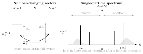
An annihilation operator maps the $N$-particle ground state into exact $N-1$ states, while a creation operator maps it into exact $N+1$ states. With energies measured relative to $\mu$, removal weight appears at $E=-\Delta_n^-$ and addition weight at $E=+\Delta_m^+$. A finite system has discrete lines; dense many-body levels can become continua in a thermodynamic limit.

Fermionic Spectral Function

Define the matrix spectral function by

$$A(E) = \frac{i}{2\pi} \left[ G^{\mathrm R}(E) - G^{\mathrm A}(E) \right].$$

For a diagonal element,

$$A_{aa}(E) = -\frac{1}{\pi} \operatorname{Im} G_{aa}^{\mathrm R}(E).$$

At zero temperature,

$$\begin{aligned} A_{ab}(E) ={}& \sum_m X_{am}^{+} X_{bm}^{+*} \delta(E-\Delta_m^+) \\ &+ \sum_n X_{an}^{-} X_{bn}^{-*} \delta(E+\Delta_n^-). \end{aligned}$$

Conversely, for complex $z$ away from the real axis,

$$G_{ab}(z) = \int_{-\infty}^{\infty} dE'\, \frac{ A_{ab}(E') }{ z-E' }.$$

The retarded boundary value is obtained with $z=E+i0^+$.

Hermiticity and positivity

The spectral matrix is Hermitian:

$$A_{ab}(E) = A_{ba}^*(E).$$

For any complex vector $v$,

$$v^\dagger A(E)v \geq 0$$

as a distribution. To see this, define

$$d^\dagger = \sum_a v_a c_a^\dagger.$$

Every Lehmann coefficient in the diagonal spectrum of $d$ is an absolute square. A negative diagonal fermionic spectral density therefore indicates a sign, continuation, normalization, or numerical-resolution problem.

Zeroth-moment sum rule

Integrating over energy and using completeness,

$$\begin{aligned} \int_{-\infty}^{\infty} dE\, A_{ab}(E) &= \left\langle \left\{ c_a,c_b^\dagger \right\} \right\rangle \\ &= \delta_{ab}. \end{aligned}$$

For one canonical orbital,

$$\int_{-\infty}^{\infty} dE\, A_{aa}(E) = 1.$$

Interactions redistribute this unit weight. They do not create extra canonical weight.

Occupied and unoccupied weight

At zero temperature, with no state pinned exactly at $E=0$,

$$n_{ab} = \int_{-\infty}^{0} dE\, A_{ab}(E).$$

Thus removal weight is occupied weight, while

$$\delta_{ab}-n_{ab} = \int_{0}^{\infty} dE\, A_{ab}(E)$$

is available addition weight.

At nonzero temperature,

$$n_{ab} = \int_{-\infty}^{\infty} dE\, f(E)A_{ab}(E),$$

where

$$f(E) = \frac{1}{ e^{\beta E}+1 }.$$

This identity separates spectral availability, $A(E)$, from equilibrium occupation, $f(E)$.

Spectral Function Versus Density of States

For a local orbital $a$, $A_{aa}(E)$ is its local single-particle spectral density. In a translation-invariant system,

$$A(\mathbf k,E) = \frac{i}{2\pi} \left[ G^{\mathrm R}(\mathbf k,E) - G^{\mathrm A}(\mathbf k,E) \right].$$

A trace such as

$$\rho_{\mathrm{sp}}(E) = \frac1L \sum_{\mathbf k} \operatorname{Tr} A(\mathbf k,E)$$

is an interacting single-particle density of states per site, with the trace taken over declared internal orbitals.

This is not the full many-body density of states,

$$\rho_{\mathrm{MB}}(\mathcal E) = \sum_r \delta(\mathcal E-E_r),$$

which counts complete many-body eigenstates in specified sectors. The two objects have different variables, normalizations, and physical questions.

Thermal Lehmann Representation

Let

$$\mathcal K|r\rangle = K_r|r\rangle, \qquad p_r = \frac{e^{-\beta K_r}}{\Xi}.$$

For fermionic annihilation operators,

$$\begin{aligned} A_{ab}(E) ={}& \sum_{r,s} \left( p_r+p_s \right) \\ &\times \langle r|c_a|s\rangle \langle s|c_b^\dagger|r\rangle \\ &\times \delta \left( E-K_s+K_r \right). \end{aligned}$$

The matrix element requires the state $|s\rangle$ to have one more particle than $|r\rangle$. The positive coefficient $p_r+p_s$ preserves fermionic spectral positivity at finite temperature.

Equilibrium greater and lesser functions satisfy

$$G_{ab}^{<}(E) = 2\pi i\, f(E) A_{ab}(E),$$

and

$$G_{ab}^{>}(E) = -2\pi i \left[ 1-f(E) \right] A_{ab}(E).$$

Consequently,

$$A_{ab}(E) = \frac{i}{2\pi} \left[ G_{ab}^{>}(E) - G_{ab}^{<}(E) \right].$$

These relations assume equilibrium and the present normalization. A driven system generally requires independent spectral and distribution information.

Free Fermion Benchmark

Consider one canonical fermionic mode with

$$\mathcal K = \xi c^\dagger c, \qquad \xi = \epsilon-\mu.$$

Its evolution is

$$c(t) = e^{-i\xi t/\hbar}c.$$

Because

$$\left\{ c,c^\dagger \right\} = 1,$$

the retarded function is

$$G^{\mathrm R}(t) = -\frac{i}{\hbar} \theta(t) e^{-i\xi t/\hbar},$$

and

$$G^{\mathrm R}(E) = \frac1{ E-\xi+i0^+ }.$$

The spectral function is

$$A(E) = \delta(E-\xi).$$

The retarded free function is independent of the occupation because the anticommutator is an operator identity. The greater and lesser functions are not:

$$G^{>}(t) = -\frac{i}{\hbar} \left( 1-f(\xi) \right) e^{-i\xi t/\hbar},$$

and

$$G^{<}(t) = \frac{i}{\hbar} f(\xi) e^{-i\xi t/\hbar}.$$

The equilibrium time-ordered function is

$$\begin{aligned} G^{\mathrm T}(E) ={}& \frac{ 1-f(\xi) }{ E-\xi+i0^+ } \\ &+ \frac{ f(\xi) }{ E-\xi-i0^+ }. \end{aligned}$$

The same pole therefore carries different boundary data depending on the physical Green function.

Quadratic Multi-Orbital Benchmark

Let

$$\mathcal K_0 = \sum_{a,b} c_a^\dagger h_{ab} c_b,$$

where $h=h^\dagger$ already includes the chemical-potential shift. If

$$h = U \operatorname{diag} \left( \xi_1,\ldots,\xi_M \right) U^\dagger,$$

then

$$G_0^{\mathrm R}(E) = \left[ (E+i0^+)I-h \right]^{-1}.$$

In components,

$$G_{0,ab}^{\mathrm R}(E) = \sum_\lambda \frac{ U_{a\lambda} U_{b\lambda}^* }{ E-\xi_\lambda+i0^+ }.$$

The spectral matrix is

$$A_{0,ab}(E) = \sum_\lambda U_{a\lambda} U_{b\lambda}^* \delta(E-\xi_\lambda).$$

Hybridization can therefore split the spectrum seen by one local orbital even without interactions. Multiple peaks alone do not prove many-body correlation.

How Interactions Redistribute Weight

Suppose an addition state decomposes schematically as

$$c_a^\dagger |\Psi_0\rangle = \sqrt Z\,|\Phi_{\mathrm{sharp}}\rangle + \sqrt{1-Z}\,|\Phi_{\mathrm{rest}}\rangle,$$

with normalized orthogonal components. The sharp state contributes pole weight $Z$ if it is an exact isolated eigenstate. The remaining weight can be spread among satellite poles or a continuum.

The residue is therefore an overlap:

$$Z = \left| \langle \Phi_{\mathrm{sharp}} | c_a^\dagger | \Psi_0 \rangle \right|^2.$$

It is not automatically one, and it is not the probability that a permanent microscopic particle has survived along a path. It measures how much the exact excitation resembles the state created by the chosen bare operator.

Interactions can produce:

• shifted coherent poles;
• several atomic or molecular addition energies;
• shake-up satellites;
• multiparticle continua;
• threshold singularities;
• vanishing pole residue even when low-energy excitations remain well defined in another language.

An arbitrarily small plotting broadening turns every delta function into a smooth peak. That visual operation does not prove a finite physical lifetime.

Poles, Continua, and Limits

For a finite closed system with a discrete spectrum, the exact Lehmann representation is a sum of real-axis delta functions. Exact eigenstates do not acquire decay widths merely because the Hamiltonian is interacting.

Smooth continua can arise when:

• the thermodynamic limit makes level spacings dense;
• an excitation couples to a continuum of multiparticle states;
• the system is genuinely open;
• disorder or ensemble averaging introduces a declared average;
• an experiment convolves the intrinsic signal with finite resolution.

These mechanisms should not be conflated.

An isolated pole of $G_{aa}^{\mathrm R}$ at $E=E_\star$ implies an exact state with nonzero overlap with $c_a^\dagger|\Psi_0\rangle$ or $c_a|\Psi_0\rangle$. The converse fails for operator-dark states. A continuum threshold can also carry important physics without an isolated pole.

Dyson Equation Preview

After choosing a reference propagator $G_0$, define the exact self-energy by

$$\left[ G^{\mathrm R}(E) \right]^{-1} = \left[ G_0^{\mathrm R}(E) \right]^{-1} - \Sigma^{\mathrm R}(E).$$

For one translation-invariant band,

$$G^{\mathrm R}(\mathbf k,E) = \frac1{ E-\xi_{\mathbf k} - \Sigma^{\mathrm R}(\mathbf k,E) }.$$

The $i0^+$ prescription is understood in the retarded boundary value. A candidate quasiparticle energy satisfies

$$E_{\mathbf k}^\star - \xi_{\mathbf k} - \operatorname{Re} \Sigma^{\mathrm R} \left( \mathbf k,E_{\mathbf k}^\star \right) = 0.$$

If the self-energy is smooth and the damping is small, the pole residue is approximately

$$Z_{\mathbf k} = \left[ 1 - \left. \frac{\partial}{ \partial E } \operatorname{Re} \Sigma^{\mathrm R} (\mathbf k,E) \right|_{E=E_{\mathbf k}^\star} \right]^{-1}.$$

Writing

$$\gamma_{\mathbf k} = -Z_{\mathbf k} \operatorname{Im} \Sigma^{\mathrm R} \left( \mathbf k,E_{\mathbf k}^\star \right),$$

one obtains the local approximation

$$A(\mathbf k,E) \simeq \frac{Z_{\mathbf k}}{\pi} \frac{ \gamma_{\mathbf k} }{ (E-E_{\mathbf k}^\star)^2 + \gamma_{\mathbf k}^2 } + A_{\mathrm{inc}}.$$

This interpretation requires an isolated, slowly varying pole region and $\gamma_{\mathbf k}\geq0$. Near thresholds, strong continua, matrix-valued crossings, zeros of $G$, or critical points, a Lorentzian quasiparticle fit can fail.

Diagrammatic Methods Preview owns how proper self-energy insertions generate Dyson’s equation and how dressed-line double counting is avoided. Spectral Functions owns line-shape analysis, linewidth conventions, and coherent-versus-incoherent weight in depth.

Equation-of-Motion Hierarchy

The retarded definition gives the exact equation

$$\begin{aligned} E G_{ab}^{\mathrm R}(E) ={}& \left\langle \left\{ c_a,c_b^\dagger \right\} \right\rangle \\ &+ G_{[c_a,\mathcal K],c_b^\dagger}^{\mathrm R}(E). \end{aligned}$$

For canonical fermions, the first term is $\delta_{ab}$. If $\mathcal K$ is quadratic,

$$\left[ c_a,\mathcal K \right] = \sum_j h_{aj}c_j,$$

so the hierarchy closes:

$$\left[ EI-h \right] G_0^{\mathrm R}(E) = I.$$

For a two-body interaction, $[c_a,\mathcal K]$ contains products such as

$$c_i^\dagger c_j c_k.$$

Its Green function couples the one-particle problem to a higher-order correlator. Commuting again produces further objects. This hierarchy is exact; a self-energy, decoupling, truncation, or diagrammatic approximation is a way of organizing or closing it, not an additional identity.

High-Energy Expansion

For complex $z$ far from the spectrum,

$$G_{ab}(z) = \frac{ \delta_{ab} }{z} + \frac{ M_{ab}^{(1)} }{z^2} + O(z^{-3}).$$

The first moment is

$$M_{ab}^{(1)} = \int dE\, E A_{ab}(E),$$

and the equation of motion gives

$$M_{ab}^{(1)} = \left\langle \left\{ [c_a,\mathcal K], c_b^\dagger \right\} \right\rangle.$$

For one free mode, $M^{(1)}=\xi$. These asymptotic coefficients are powerful checks on exact diagonalization, impurity solvers, moment expansions, and numerical continuation. Sum Rules develops the systematic hierarchy and distinguishes graded single-particle moments from observable response moments.

Bosonic Single-Particle Functions

For canonical bosons,

$$\left[ b_a,b_b^\dagger \right] = \delta_{ab},$$

and the retarded function uses a commutator:

$$D_{ab}^{\mathrm R}(t) = -\frac{i}{\hbar} \theta(t) \left\langle \left[ b_a(t),b_b^\dagger \right] \right\rangle.$$

The zeroth moment remains

$$\int dE\, A_{ab}^{(b)}(E) = \delta_{ab}.$$

The thermal Lehmann coefficient is now a difference:

$$\begin{aligned} A_{ab}^{(b)}(E) ={}& \sum_{r,s} \left( p_r-p_s \right) \\ &\times \langle r|b_a|s\rangle \langle s|b_b^\dagger|r\rangle \\ &\times \delta(E-K_s+K_r). \end{aligned}$$

Unlike the normal fermionic spectral matrix, a bosonic commutator spectrum is not positive semidefinite at every energy. Negative-frequency weight can carry the opposite sign while the integrated commutator sum rule remains correct.

Condensates and broken symmetry

If

$$\left\langle b_a \right\rangle \ne 0,$$

the time-ordered product contains a disconnected condensate contribution. It is often cleaner to define

$$\delta b_a = b_a - \left\langle b_a \right\rangle$$

and build connected fluctuation Green functions.

Pairing or broken $U(1)$ symmetry also motivates Nambu matrices containing normal and anomalous correlators such as

$$\left\langle \mathcal T b_a(t)b_b(0) \right\rangle.$$

Their spectral normalization involves a particle–hole metric rather than ordinary scalar positivity. A scalar fermionic sum rule should not be transferred blindly to a bosonic or Nambu matrix.

Single-Particle Green Function Versus Response

The fermionic retarded single-particle function contains an anticommutator:

$$G_{ab}^{\mathrm R}(t) \propto \theta(t) \left\langle \left\{ c_a(t),c_b^\dagger \right\} \right\rangle.$$

By contrast, the Kubo susceptibility of physical observables $A$ and $B$ contains an ordinary commutator:

$$\chi_{AB}^{\mathrm R}(t) = -\frac{i}{\hbar} \theta(t) \left\langle \left[ A(t),B \right] \right\rangle.$$

The two objects answer different questions:

Object	Changes particle number?	Bracket	Typical role
fermion $G^{\mathrm R}$	by one at each insertion	anticommutator	addition and removal spectrum
boson $D^{\mathrm R}$	by one at each insertion	commutator	bosonic propagation spectrum
susceptibility $\chi^{\mathrm R}$	usually number preserving	commutator	response to a classical source
structure factor $S(\mathbf q,E)$	usually number preserving	ordinary ordered product	scattering intensity

A fermionic Green function can be generated formally by Grassmann sources, but it is not an ordinary response to a classical laboratory force. Calling every retarded object a susceptibility erases this distinction.

Matsubara Green Function Preview

Imaginary time is defined on

$$0 \leq \tau \lt \beta\hbar,$$

with

$$c_a(\tau) = e^{\tau\mathcal K/\hbar} c_a e^{-\tau\mathcal K/\hbar}.$$

The fermionic imaginary-time Green function is

$$\mathcal G_{ab}(\tau) = - \left\langle \mathcal T_\tau c_a(\tau)c_b^\dagger(0) \right\rangle.$$

It is antiperiodic:

$$\mathcal G_{ab} (\tau+\beta\hbar) = - \mathcal G_{ab}(\tau).$$

Therefore its angular Matsubara frequencies are

$$\omega_n = \frac{ (2n+1)\pi }{ \beta\hbar },$$

or, in energy units,

$$\nu_n = \hbar\omega_n = \frac{ (2n+1)\pi }{ \beta }.$$

Using the energy-frequency notation,

$$\mathcal G_{ab}(i\nu_n) = \frac1\hbar \int_0^{\beta\hbar} d\tau\, e^{i\nu_n\tau/\hbar} \mathcal G_{ab}(\tau).$$

The spectral representation is

$$\mathcal G_{ab}(i\nu_n) = \int_{-\infty}^{\infty} dE\, \frac{ A_{ab}(E) }{ i\nu_n-E }.$$

For one free mode,

$$\mathcal G_0(i\nu_n) = \frac1{ i\nu_n-\xi }.$$

Bosonic imaginary-time functions are periodic and use

$$\nu_n^{(b)} = \frac{ 2\pi n }{ \beta }.$$

Finite-Temperature QM Overview gives the common equilibrium roadmap from the Gibbs operator through KMS cyclicity, boundary conditions, Matsubara modes, spectral data, and path integrals. Bosonic and Fermionic Matsubara Frequencies owns the grids, units, index arithmetic, and zero-mode conventions. Thermal Green Functions owns the detailed imaginary-time signs, one-sided limits, contact terms, and free fermion and boson benchmarks. Spectral Representation owns the general thermal Lehmann kernel, Matsubara Cauchy transform, and retarded boundary bridge. Matsubara Formalism Preview owns the compact-time transform, sum measures, convergence prescriptions, and QFT handoff. This page retains the single-particle addition, removal, and spectral conventions.

Analytic Continuation

The same spectral density defines an analytic function

$$G(z) = \int dE'\, \frac{ A(E') }{ z-E' }.$$

Matsubara data sample it at

$$z=i\nu_n,$$

whereas the retarded function is the boundary value

$$G^{\mathrm R}(E) = G(E+i0^+).$$

This motivates the formal rule

$$i\nu_n \longrightarrow E+i0^+.$$

The rule is applied to the analytic function after frequency sums and algebra are complete. It is not a license to substitute into an arbitrary discrete table.

Exact values at all Matsubara frequencies plus suitable analyticity and asymptotic information determine the continuation in principle. Reconstructing a real-frequency spectrum from finite noisy imaginary-time data is nevertheless ill conditioned: many spectra can fit the data within uncertainty. Regularization, priors, resolution tests, and sum rules must be reported. Analytic Continuation owns the covariance-aware inverse problem and its method-specific limitations.

What Experiments Probe

Single-particle spectroscopy couples to particle addition or removal, but measured intensity includes more than $A$.

Removal probes

Photoemission and radio-frequency ejection can be schematically sensitive to

$$I_{\mathrm{rem}} \propto \left| M \right|^2 f(E) A(\mathbf k,E),$$

followed by kinematic factors, final-state effects, backgrounds, and instrumental convolution.

Addition probes

Inverse photoemission or injection-type probes can instead emphasize

$$I_{\mathrm{add}} \propto \left| M \right|^2 \left[ 1-f(E) \right] A(\mathbf k,E).$$

Local tunneling

Under controlled assumptions, a tunneling conductance can track a convolution of tip and sample local spectral densities. Temperature, matrix elements, voltage division, nonequilibrium occupations, and junction structure matter. The statement

$$\frac{dI}{dV} \propto \rho_{\mathrm{sample}}(eV)$$

is a useful limit, not a universal identity.

Scanning Tunneling Microscopy and Spectroscopy develops the corresponding junction model, acquisition protocol, local maps, and experimental systematics.

Scattering experiments that transfer momentum and energy without adding or removing a constituent generally probe structure factors or susceptibilities instead. A peak in $S(\mathbf q,E)$ and a peak in $A(\mathbf k,E)$ need not represent the same operator channel.

Numerical Evaluation

Exact diagonalization

Exact diagonalization can evaluate the Lehmann sums directly. For a finite Hilbert space the spectrum is discrete. A plotted broadening

$$\delta(E-E_m) \longrightarrow \frac1\pi \frac{ \eta }{ (E-E_m)^2+\eta^2 }$$

should be labeled as numerical resolution unless a physical bath or limiting procedure justifies $\eta$ as a lifetime.

Krylov and Lanczos continued fractions can evaluate matrix elements of

$$\frac1{ E+i\eta-\mathcal K }$$

without diagonalizing every state. Convergence in Krylov dimension and $\eta$ must both be checked.

Real-time evolution

One may create

$$c_b^\dagger |\Psi_0\rangle$$

or

$$c_a |\Psi_0\rangle,$$

evolve the state, and Fourier transform the overlap. Finite duration sets energy resolution, windowing changes line shape, and entanglement growth can limit reachable times.

Imaginary-time methods

Quantum Monte Carlo and thermal tensor-network methods often produce $\mathcal G(\tau)$ or $\mathcal G(i\nu_n)$. These quantities can be accurate even when the inferred real-frequency $A(E)$ is not unique. A continuation result should be tested against:

• covariance-aware data errors;
• the zeroth and known higher moments;
• positivity where applicable;
• synthetic-data resolution;
• dependence on the continuation prior or regularizer.

Impurity and embedding solvers

Impurity methods return local Green functions and self-energies under model-specific self-consistency conditions. Causality, high-frequency moments, particle number, and convergence of the self-consistency loop are essential checks. The returned spectrum is not automatically a momentum-resolved lattice spectrum.

Finite Size, Thermodynamic Limits, and Widths

Three limits frequently fail to commute:

$$L\to\infty, \qquad t_{\max}\to\infty, \qquad \eta\to0^+.$$

For a finite system, taking $\eta\to0^+$ first reveals exact delta functions. Taking $L\to\infty$ can create a continuum before $\eta$ is removed. A finite observation time produces a convolution whose width scales with the chosen window.

When quoting a linewidth, state whether it comes from:

• the imaginary part of a controlled retarded self-energy;
• coupling to an external environment;
• disorder or ensemble averaging;
• finite observation time;
• instrumental resolution;
• an artificial numerical regulator.

Only the first three can represent intrinsic or declared physical broadening of the modeled system.

Validation Checklist

Before trusting a single-particle Green-function calculation, check:

1. Generator: Is time evolution defined with $H$ or $H-\mu\hat N$?
2. Ordering: Is the function greater, lesser, retarded, advanced, time ordered, or imaginary time?
3. Statistics: Is the bracket a commutator or anticommutator?
4. Units: Is the frequency variable an energy or an angular frequency?
5. Indices: Which site, orbital, spin, band, or Nambu basis is used?
6. Normalization: Does $\int dE\,A_{ab}(E)=\delta_{ab}$ hold for canonical fermions?
7. Positivity: Is the diagonal normal fermionic spectral density nonnegative?
8. Occupancy: Does $\int dE\,f(E)A(E)$ reproduce the one-body density matrix?
9. Asymptotics: Does $zG(z)\to I$ at large $\lvert z\rvert$?
10. Causality: Is $G^{\mathrm R}$ analytic in the upper half-plane?
11. Finite size: Are delta functions, level spacings, and broadening stated honestly?
12. Approximation: Are self-energy and vertex approximations compatible with the claimed conservation laws?

Common Mistakes

• Treating a single-particle Green function as the amplitude for one labeled particle to follow a path.
• Forgetting that creation and annihilation operators connect different particle-number sectors.
• Calling the full many-body density of states a single-particle spectral function.
• Using a commutator for a normal fermionic retarded propagator.
• Using an anticommutator for a bosonic response without stating a nonstandard convention.
• Mixing evolution with $H$ and $H-\mu\hat N$ without shifting frequency.
• Calling a variable $\omega$ while switching silently between energy and angular-frequency units.
• Assuming the retarded and time-ordered $i0$ prescriptions are identical.
• Interpreting every pole as a stable quasiparticle or every broad peak as a finite lifetime.
• Ignoring operator selection rules when an expected excitation is absent.
• Violating fermionic positivity or the unit spectral sum rule and blaming interactions.
• Treating a plotting parameter $\eta$ as a measured decay rate.
• Performing $i\nu_n\to E+i0^+$ before constructing the analytic function.
• Claiming a unique real-frequency spectrum from finite noisy imaginary-time data.
• Applying scalar positivity to bosonic commutator or Nambu spectral matrices.
• Equating a single-particle Green function with a Kubo susceptibility or structure factor.

Reliable Workflow

1. Specify the state, ensemble, particle-number symmetry, and generator.
2. Declare the operator basis and statistics.
3. Write the exact real-time or imaginary-time definition before Fourier transforming.
4. Fix energy versus angular-frequency units.
5. Use a Lehmann representation to identify sectors, signs, and support.
6. Check canonical discontinuities, positivity, and spectral moments.
7. Separate exact poles from numerical or instrumental broadening.
8. Introduce a self-energy only after defining the reference propagator.
9. Validate analytic continuation against moments and synthetic resolution.
10. Translate to an experiment only after including matrix elements, occupations, kinematics, and resolution.

Exercises

Exercise 1: Free orbital

For

$$\mathcal K = \xi c^\dagger c,$$

derive $c(t)$, $G^{\mathrm R}(t)$, $G^{\mathrm R}(E)$, and $A(E)$.

Solution

The commutator is

$$\left[ c,\mathcal K \right] = \xi c.$$

The Heisenberg equation gives

$$i\hbar \frac{dc}{dt} = \xi c,$$

so

$$c(t) = e^{-i\xi t/\hbar}c.$$

Using $\{c,c^\dagger\}=1$,

$$G^{\mathrm R}(t) = -\frac{i}{\hbar} \theta(t) e^{-i\xi t/\hbar}.$$

The transform is

$$G^{\mathrm R}(E) = \frac1{ E-\xi+i0^+ }.$$

Therefore

$$A(E) = -\frac1\pi \operatorname{Im} G^{\mathrm R}(E) = \delta(E-\xi).$$

Exercise 2: Lehmann sum rule

Use the ground-state addition and removal amplitudes to prove

$$\int dE\, A_{ab}(E) = \delta_{ab}.$$

Solution

Integrating the Lehmann representation gives

$$\begin{aligned} \int dE\, A_{ab}(E) ={}& \sum_m X_{am}^{+} X_{bm}^{+*} \\ &+ \sum_n X_{an}^{-} X_{bn}^{-*}. \end{aligned}$$

Completeness in the $N+1$ sector turns the first term into

$$\langle \Psi_0^N | c_a c_b^\dagger | \Psi_0^N \rangle.$$

Completeness in the $N-1$ sector turns the second into

$$\langle \Psi_0^N | c_b^\dagger c_a | \Psi_0^N \rangle.$$

Their sum is

$$\left\langle \left\{ c_a,c_b^\dagger \right\} \right\rangle = \delta_{ab}.$$

Exercise 3: Chemical-potential window

Show that

$$\mu_N^- \lt \mu \lt \mu_N^+$$

implies positive lowest addition and removal costs. Explain where their spectral peaks occur.

Solution

The lowest addition cost is

$$\Delta_0^+ = E_0^{N+1} - E_0^N - \mu = \mu_N^+-\mu.$$

The upper inequality gives $\Delta_0^+\gt0$. The lowest removal cost is

$$\Delta_0^- = E_0^{N-1} - E_0^N + \mu = \mu-\mu_N^-,$$

which is positive by the lower inequality.

Addition appears at

$$E=+\Delta_0^+,$$

while removal appears at

$$E=-\Delta_0^-.$$

Excited states in the neighboring sectors produce peaks farther from zero.

Exercise 4: Shared spectral weight

Suppose $c|\Psi_0\rangle=0$ and the normalized addition state satisfies

$$c^\dagger|\Psi_0\rangle = \sqrt Z\,|1\rangle + \sqrt{1-Z}\,|2\rangle,$$

where $|1\rangle$ and $|2\rangle$ are orthonormal exact eigenstates with positive addition energies $E_1$ and $E_2$. Find the addition spectral function and its first two basic sum checks.

Solution

The overlap weights are $Z$ and $1-Z$, so

$$A(E) = Z\delta(E-E_1) + (1-Z)\delta(E-E_2).$$

Its zeroth moment is

$$\int dE\,A(E) = Z+(1-Z) = 1.$$

Its first moment is

$$\int dE\, E A(E) = Z E_1 + (1-Z)E_2.$$

The two exact states share the canonical orbital’s unit spectral weight.

Exercise 5: Retarded versus time ordered

For a free occupied mode with $\xi\lt0$ at zero temperature, compare $G^{\mathrm R}(E)$ and $G^{\mathrm T}(E)$.

Solution

The retarded function follows from the anticommutator and is

$$G^{\mathrm R}(E) = \frac1{ E-\xi+i0^+ }.$$

Because the mode is occupied, its time-ordered contribution is a removal or hole term:

$$G^{\mathrm T}(E) = \frac1{ E-\xi-i0^+ }.$$

The pole position is the same, but it is approached from the opposite side of the real axis. Time ordering and retardation are therefore not interchangeable.

Exercise 6: Fermionic Matsubara frequencies

Show that antiperiodicity over $\beta\hbar$ selects

$$\nu_n = \frac{ (2n+1)\pi }{ \beta }.$$

Solution

A Fourier basis function is

$$e^{-i\nu\tau/\hbar}.$$

Antiperiodicity requires

$$e^{-i\nu(\tau+\beta\hbar)/\hbar} = - e^{-i\nu\tau/\hbar}.$$

After canceling the common factor,

$$e^{-i\beta\nu} = -1.$$

Hence

$$\beta\nu = (2n+1)\pi,$$

which gives the stated fermionic energy frequencies. Dividing by $\hbar$ gives the corresponding angular frequencies.

Exercise 7: Matrix positivity

Prove that the normal fermionic spectral matrix is positive semidefinite by considering

$$d^\dagger = \sum_a v_a c_a^\dagger.$$

Solution

The spectral function associated with $d$ is

$$A_d(E) = \sum_{a,b} v_a^* A_{ab}(E) v_b = v^\dagger A(E)v.$$

In the Lehmann representation, every addition term has weight

$$\left| \langle m,N+1 | d^\dagger | \Psi_0^N \rangle \right|^2,$$

and every removal term has weight

$$\left| \langle n,N-1 | d | \Psi_0^N \rangle \right|^2.$$

All coefficients multiplying delta functions are nonnegative. Therefore

$$v^\dagger A(E)v \geq 0$$

for every $v$, in the distributional sense.

Exercise 8: Choose the correct correlator

For each question, choose a single-particle Green function, a density structure factor, or a Kubo susceptibility:

1. What energies are required to add an electron with momentum $\mathbf k$?
2. What momentum and energy are transferred by density scattering?
3. What magnetization is induced by a weak magnetic field?

Solution

1. Use the electron-addition part of the single-particle spectral function $A(\mathbf k,E)$. Its operator insertions change particle number by one.
2. Use the dynamic density structure factor $S_n(\mathbf q,E)$. It is a number-preserving density–density spectrum with the scattering transfer variables.
3. Use the retarded magnetic susceptibility from the Kubo formula. It relates a weak applied field to the induced magnetization.

The three objects can contain related excitations, but their operators, matrix elements, normalizations, and experimental couplings differ.

Cross-Links

• Time-Dependent Correlations — ordinary two-time spectra, stationarity, and finite-time behavior.
• Retarded and Advanced Response — commutator response, adjoint identities, analyticity, and dispersion relations.
• Structure Factors — number-preserving momentum–energy spectra and scattering probes.
• Spectral Functions — cross-channel line shapes, quasiparticle peaks, linewidths, and measured intensity.
• Kubo Formula — retarded response of observables to classical sources.
• Sum Rules — general nested-commutator moments and cross-channel diagnostics.
• Field Operators in Many-Body Models — creation, annihilation, basis, and normalization conventions.
• Grand-Canonical Ensemble — the generator $H-\mu\hat N$ and equilibrium weights.
• Ideal Fermi Gas — free occupations, Fermi surface, and thermodynamics.
• Anderson Impurity Model Preview — resonant-level and correlated atomic spectral examples.
• Diagrammatic Methods Preview — self-energy, Dyson resummation, and diagram conventions.
• Matsubara Formalism Preview — graded thermal boundaries, discrete transforms, and frequency sums.
• Bosonic and Fermionic Matsubara Frequencies — formulas, units, index pairing, zero modes, and numerical grids.
• Thermal Green Functions — imaginary-time signs, contact jumps, occupations, and exact free-mode benchmarks.
• Superconducting Proximity Effect — applies equilibrium Nambu Green functions to spatial anomalous propagation, self-consistent interfaces, and controlled quasiclassical reductions; this page retains the generic correlator, spectrum, and analytic conventions.
• Spectral Representation — thermal Lehmann weights, Euclidean kernels, Matsubara transforms, and retarded boundary values.
• What Is a Green Function? — inverse kernels and boundary prescriptions.
• Retarded and Advanced Green Functions — causal support, analyticity, and $i0$ rules.
• Spectral Representation of Green Functions — spectral-theorem foundations for resolvents.
• Green Functions from QM to QFT — translation to field propagators.
• Correlation Functions in Path Integrals — ordered insertions and source methods.
• Wick’s Theorem Preview — contractions around Gaussian references.
• Correlation Functions Formula Card — compact ordering conventions.
• Fourier-Transform Conventions — energy and angular-frequency transforms.

References

1. H. Lehmann, “On the Properties of Propagation Functions and Renormalization Constants of Quantized Fields”, Il Nuovo Cimento 11, 342–357 (1954).
2. T. Matsubara, “A New Approach to Quantum-Statistical Mechanics”, Progress of Theoretical Physics 14, 351–378 (1955).
3. P. C. Martin and J. Schwinger, “Theory of Many-Particle Systems. I”, Physical Review 115, 1342–1373 (1959).
4. F. J. Dyson, “The Radiation Theories of Tomonaga, Schwinger, and Feynman”, Physical Review 75, 486–502 (1949).
5. J. M. Luttinger and J. C. Ward, “Ground-State Energy of a Many-Fermion System. II”, Physical Review 118, 1417–1427 (1960).
6. G. Baym and L. P. Kadanoff, “Conservation Laws and Correlation Functions”, Physical Review 124, 287–299 (1961).
7. L. Hedin, “New Method for Calculating the One-Particle Green’s Function with Application to the Electron-Gas Problem”, Physical Review 139, A796–A823 (1965).
8. A. L. Fetter and J. D. Walecka, Quantum Theory of Many-Particle Systems, Dover (2003).
9. J. W. Negele and H. Orland, Quantum Many-Particle Systems, Westview Press (1998).
10. G. D. Mahan, Many-Particle Physics, 3rd ed., Springer (2000).
11. P. Coleman, Introduction to Many-Body Physics, Cambridge University Press (2015).
12. A. A. Abrikosov, L. P. Gorkov, and I. E. Dzyaloshinski, Methods of Quantum Field Theory in Statistical Physics, Dover (1975).