Thermal Green Functions

A thermal Green function packages equilibrium propagation, occupation, operator statistics, and equal-time algebra into one imaginary-time two-point function.

For a normal fermionic single-particle channel,

$$\mathcal G_{ab}(\tau) = - \left\langle \mathcal T_\tau c_a(\tau)c_b^\dagger(0) \right\rangle_\beta.$$

The same definition simultaneously knows:

• that $c_a$ changes particle number;
• that exchanging two odd operators contributes a minus sign;
• that the thermal interval has length $\beta\hbar$;
• that the function is antiperiodic;
• that its $0^-$ limit is the one-body density matrix;
• that its $0^+-0^-$ jump is fixed by the canonical anticommutator.

Those facts are not optional decorations. They are the checks that distinguish a valid thermal propagator from a formula with the right denominator but the wrong physics.

Canonical Scope

This page is the canonical home for:

• the definition of equilibrium imaginary-time two-point functions;
• graded imaginary-time ordering as applied to thermal Green functions;
• the distinction between exchange signs and conventional overall signs;
• normal fermionic and bosonic single-particle propagators;
• one-sided equal-time limits and contact terms;
• occupation matrices extracted from $0^-$;
• exact free fermion and free boson time-domain benchmarks;
• the harmonic-oscillator coordinate correlator as a contrasting bosonic convention;
• quadratic many-orbital Green functions;
• equation-of-motion and high-frequency checks;
• practical validation of imaginary-time data.

Neighboring pages retain separate ownership:

• Imaginary Time develops the semigroup, thermal trace, open kernels, and closed thermal circle.
• Bosonic and Fermionic Matsubara Frequencies owns the allowed grids, units, index symmetries, and finite cutoffs.
• Matsubara Formalism Preview owns the complete transform, loop-sum, convergence, and calculation workflow.
• Green Functions in Many-Body QM owns addition and removal sectors, Lehmann representations, spectral normalization, and real-frequency single-particle interpretation.
• Spectral Representation owns the general thermal Lehmann kernel, graded spectral density, Matsubara–retarded bridge, and static bosonic term.
• Diagrammatic Methods Preview owns propagator lines, vertices, self-energies, and diagrammatic bookkeeping.
• Kubo Formula owns causal response to an applied source.

Convention Ledger

Equilibrium generator

Use one generator consistently in the density operator and in imaginary-time evolution:

$$\rho_\beta = \frac{ e^{-\beta\mathcal K} }{ \mathcal Z }, \qquad \mathcal Z = \operatorname{Tr} e^{-\beta\mathcal K}.$$

For a grand-canonical state,

$$\mathcal K = H-\mu N.$$

Imaginary-time operators are

$$A(\tau) = e^{\tau\mathcal K/\hbar} A e^{-\tau\mathcal K/\hbar}.$$

Using $H$ in this evolution while retaining $H-\mu N$ in the Gibbs weight changes where $\mu$ appears. Either convention can be translated into the other, but they must not be mixed silently.

Thermal interval

Write

$$L_\tau := \beta\hbar, \qquad 0 \leq \tau \lt L_\tau.$$

The notation keeps $\tau$ in time units and $\beta$ in inverse-energy units.

Matsubara-energy transform

For a periodic or antiperiodic function $\mathcal C(\tau)$, this page uses

$$\mathcal C(i\zeta_n) = \frac1\hbar \int_0^{L_\tau} d\tau\, e^{i\zeta_n\tau/\hbar} \mathcal C(\tau),$$

with inverse

$$\mathcal C(\tau) = \frac1\beta \sum_n e^{-i\zeta_n\tau/\hbar} \mathcal C(i\zeta_n).$$

The symbol $\zeta_n$ is generic. For a bosonic channel,

$$\zeta_n = \Omega_m = \frac{2\pi m}{\beta}.$$

For a fermionic channel,

$$\zeta_n = \nu_n = \frac{(2n+1)\pi}{\beta}.$$

What Is Being Correlated?

A two-point function is not specified by the words “Green function” alone. One must state:

1. the two operators;
2. the equilibrium ensemble;
3. the ordering prescription;
4. the overall prefactor;
5. the operator parity;
6. whether disconnected expectation values have been subtracted;
7. whether the variable is time, angular frequency, or energy.

Examples include:

Object	Operators	Common definition	Boundary class
fermion propagator	$c_a$, $c_b^\dagger$	$-\langle\mathcal T_\tau c_a c_b^\dagger\rangle$	antiperiodic
boson propagator	$b_a$, $b_b^\dagger$	$-\langle\mathcal T_\tau b_a b_b^\dagger\rangle$	periodic
coordinate correlator	$q$, $q$	$+\langle\mathcal T_\tau q q\rangle$	periodic
density correlator	$\delta n$, $\delta n$	$+\langle\mathcal T_\tau\delta n\,\delta n\rangle$	periodic
spin correlator	$\delta S^\alpha$, $\delta S^\beta$	convention dependent	periodic
pair correlator	$\Delta$, $\Delta^\dagger$	convention dependent	periodic

The first two rows share a conventional leading minus sign, but their exchange signs differ. The next rows illustrate that a bosonic or even channel need not use that leading minus sign at all.

Graded Imaginary-Time Ordering

Let $A$ and $B$ have definite fermion parities

$$p_A, p_B \in \{0,1\}.$$

Imaginary-time ordering is

$$\begin{aligned} \mathcal T_\tau A(\tau)B(\tau') ={}& \theta(\tau-\tau') \\ &\quad\times A(\tau)B(\tau') \\ &+ (-1)^{p_Ap_B} \theta(\tau'-\tau) \\ &\quad\times B(\tau')A(\tau). \end{aligned}$$

When both operators are odd, reversing them contributes a minus sign. If either is even, no graded exchange sign appears.

For a channel-dependent overall convention $s_{AB}$, define

$$\mathcal C_{AB}(\tau-\tau') = s_{AB} \left\langle \mathcal T_\tau A(\tau)B(\tau') \right\rangle_\beta.$$

The fixed sign $s_{AB}$ and the exchange sign $(-1)^{p_Ap_B}$ have different origins:

• $s_{AB}$ is chosen by convention;
• $(-1)^{p_Ap_B}$ follows from graded operator algebra.

Changing the first does not change the thermal boundary class. Dropping the second changes the physics.

Piecewise form

Set $\tau'=0$ and suppose the two insertions have the same parity $p$. With

$$\eta_p = (-1)^p,$$

the ordered correlator is

$$\mathcal C_{AB}(\tau) = \begin{cases} s_{AB} \langle A(\tau)B(0)\rangle_\beta, & \tau>0, \\[4pt] s_{AB}\eta_p \langle B(0)A(\tau)\rangle_\beta, & \tau<0. \end{cases}$$

The two branches contain different operator products. At finite temperature both may be nonzero because the initial thermal state need not be the ground state or the vacuum.

Stationarity and Time Differences

Since

$$[\rho_\beta,\mathcal K] = 0,$$

an equilibrium two-point function is invariant under a common imaginary-time translation:

$$\mathcal C_{AB}(\tau,\tau') = \mathcal C_{AB}(\tau-\tau',0).$$

This statement assumes:

• a time-independent equilibrium generator;
• no explicit imaginary-time dependence in the operators beyond Heisenberg evolution;
• a well-defined thermal trace or equilibrium state.

A driven state, a transient preparation, or a source varying around the thermal contour generally depends on both time arguments separately. Matsubara frequency is then not a complete label.

Thermal Boundary Conditions

KMS Condition Preview owns the analytic boundary relation by which trace cyclicity moves an insertion around the thermal circle. Graded ordering supplies the sign needed to restore the chosen order. For a two-point channel generated by parity $p$,

$$\mathcal C_p(\tau+L_\tau) = (-1)^p \mathcal C_p(\tau).$$

Thus:

$$\begin{aligned} \mathcal C_{\mathrm B}(\tau+L_\tau) &= \mathcal C_{\mathrm B}(\tau), \\ \mathcal C_{\mathrm F}(\tau+L_\tau) &= - \mathcal C_{\mathrm F}(\tau). \end{aligned}$$

The sign is assigned by the parity of the complete operator channel:

• $c_a$ is odd, so a normal fermion propagator is antiperiodic;
• $b_a$ is even under fermion parity, so a boson propagator is periodic;
• $c_a^\dagger c_b$ is even, so a density correlator is periodic;
• $c_\downarrow c_\uparrow$ is even, so a pair correlator is periodic.

Antiperiodicity is a property of the ordered thermal correlator. It does not say that a physical fermion state acquires a minus sign after an elapsed laboratory time $\beta\hbar$.

Normal Single-Particle Functions

Fermions

For canonical fermions,

$$\left\{ c_a,c_b^\dagger \right\} = \delta_{ab},$$

define

$$\mathcal G_{ab}(\tau) = - \left\langle \mathcal T_\tau c_a(\tau)c_b^\dagger(0) \right\rangle_\beta.$$

Its branches are

$$\mathcal G_{ab}(\tau) = \begin{cases} - \langle c_a(\tau)c_b^\dagger(0)\rangle_\beta, & \tau>0, \\[4pt] + \langle c_b^\dagger(0)c_a(\tau)\rangle_\beta, & \tau<0. \end{cases}$$

The plus sign on the negative-time branch results from multiplying the conventional overall minus by the odd-operator exchange minus.

Bosons

For canonical bosons,

$$\left[ b_a,b_b^\dagger \right] = \delta_{ab},$$

a common nonrelativistic convention is

$$\mathcal D_{ab}(\tau) = - \left\langle \mathcal T_\tau b_a(\tau)b_b^\dagger(0) \right\rangle_\beta.$$

The branches are

$$\mathcal D_{ab}(\tau) = \begin{cases} - \langle b_a(\tau)b_b^\dagger(0)\rangle_\beta, & \tau>0, \\[4pt] - \langle b_b^\dagger(0)b_a(\tau)\rangle_\beta, & \tau<0. \end{cases}$$

There is no exchange minus because bosonic operators are even. The leading minus remains only because this definition chose it.

Some atomic, condensed-matter, and field-theory texts define bosonic propagators with different overall signs or factors of $\hbar$. A formula should be compared only after its definition and transform pair are aligned.

Equal-Time Limits and Contact Terms

The value at exactly $\tau=0$ is less informative than the one-sided limits. Define the fermionic one-body density matrix

$$\rho_{ab}^{(1)} := \left\langle c_b^\dagger c_a \right\rangle_\beta.$$

Then

$$\begin{aligned} \mathcal G_{ab}(0^-) &= \rho_{ab}^{(1)}, \\ \mathcal G_{ab}(0^+) &= - \left( \delta_{ab} - \rho_{ab}^{(1)} \right). \end{aligned}$$

Their difference is the canonical contact term:

$$\mathcal G_{ab}(0^+) - \mathcal G_{ab}(0^-) = - \delta_{ab}.$$

For bosons, let

$$n_{ab}^{(b)} := \left\langle b_b^\dagger b_a \right\rangle_\beta.$$

The same leading-minus convention gives

$$\begin{aligned} \mathcal D_{ab}(0^-) &= - n_{ab}^{(b)}, \\ \mathcal D_{ab}(0^+) &= - \left( \delta_{ab} + n_{ab}^{(b)} \right), \end{aligned}$$

and therefore

$$\mathcal D_{ab}(0^+) - \mathcal D_{ab}(0^-) = - \delta_{ab}.$$

The equal-time jumps look identical in this convention, but their boundary gluing differs:

• the fermion propagator is antiperiodic;
• the boson propagator is periodic.

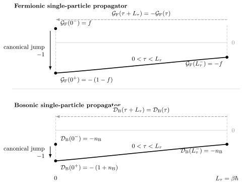
Schematic free-mode propagators on $0<\tau<L_\tau$. The canonical jump is fixed by the anticommutator or commutator. The thermal seam is separate: $\mathcal G_{\mathrm F}$ changes sign across the seam, whereas $\mathcal D_{\mathrm B}$ does not.

Occupations from frequency data

Using the inverse transform, the fermionic density matrix is

$$\rho_{ab}^{(1)} = \lim_{\epsilon\downarrow0} \frac1\beta \sum_n e^{i\nu_n\epsilon/\hbar} \mathcal G_{ab}(i\nu_n).$$

The factor $e^{i\nu_n\epsilon/\hbar}$ specifies the $0^-$ limit. Omitting it from a conditionally convergent sum can return an ambiguous midpoint rather than the occupation.

For the bosonic leading-minus convention,

$$n_{ab}^{(b)} = - \lim_{\epsilon\downarrow0} \frac1\beta \sum_m e^{i\Omega_m\epsilon/\hbar} \mathcal D_{ab}(i\Omega_m).$$

Matsubara Formalism Preview develops these convergence prescriptions in detail.

Free Fermion Mode

Consider one canonical fermion with

$$\mathcal K = \xi c^\dagger c, \qquad \xi = \epsilon-\mu.$$

Its partition function and occupation are

$$\begin{aligned} \mathcal Z_{\mathrm F} &= 1+e^{-\beta\xi}, \\ f(\xi) &= \frac1{ e^{\beta\xi}+1 }. \end{aligned}$$

The imaginary-time equation of motion gives

$$c(\tau) = e^{-\xi\tau/\hbar}c.$$

Positive-time branch

For

$$0 \lt \tau \lt L_\tau,$$

the operator order is already correct:

$$\begin{aligned} \mathcal G_{\mathrm F}(\tau) &= - e^{-\xi\tau/\hbar} \langle cc^\dagger\rangle_\beta \\ &= - \left[ 1-f(\xi) \right] e^{-\xi\tau/\hbar}. \end{aligned}$$

Negative-time branch

For

$$-L_\tau \lt \tau \lt 0,$$

graded ordering reverses the odd operators:

$$\begin{aligned} \mathcal G_{\mathrm F}(\tau) &= + e^{-\xi\tau/\hbar} \langle c^\dagger c\rangle_\beta \\ &= f(\xi) e^{-\xi\tau/\hbar}. \end{aligned}$$

Both branches matter at finite temperature. The positive-time branch carries the probability that the mode is empty, while the negative-time branch carries the probability that it is occupied.

Antiperiodicity check

The Fermi function obeys

$$\left[ 1-f(\xi) \right] e^{-\beta\xi} = f(\xi).$$

Therefore,

$$\mathcal G_{\mathrm F} (\tau+L_\tau) = - \mathcal G_{\mathrm F}(\tau).$$

At the seam,

$$\begin{aligned} \mathcal G_{\mathrm F}(0^-) &= f(\xi), \\ \mathcal G_{\mathrm F}(0^+) &= - \left[ 1-f(\xi) \right], \\ \mathcal G_{\mathrm F}(L_\tau^-) &= - f(\xi). \end{aligned}$$

The first and third values are related by antiperiodicity. The first and second differ by the canonical jump.

Frequency-domain result

For a fermionic Matsubara energy $\nu_n$,

$$e^{i\beta\nu_n} = -1.$$

Transforming the positive-time branch gives

$$\begin{aligned} \mathcal G_{\mathrm F}(i\nu_n) ={}& - \left[ 1-f(\xi) \right] \\ &\times \frac{ e^{\beta(i\nu_n-\xi)}-1 }{ i\nu_n-\xi } \\ ={}& \frac1{ i\nu_n-\xi }. \end{aligned}$$

The explicit occupation factor cancels against the thermal endpoint factor. Temperature remains encoded in the discrete values of $\nu_n$ and reappears when the inverse transform reconstructs the two time-domain branches.

Limiting checks

If $\xi>0$ and $T\to0$, then

$$f(\xi) \longrightarrow 0,$$

so positive imaginary time describes adding a particle to an empty mode.

If $\xi<0$ and $T\to0$, then

$$f(\xi) \longrightarrow 1,$$

so the positive-time branch vanishes and the negative-time branch records removal from an occupied mode.

At $\xi=0$,

$$f(0) = \frac12,$$

and the propagator is constant on the open interval:

$$\mathcal G_{\mathrm F}(\tau) = - \frac12, \qquad 0<\tau<L_\tau.$$

It still has an equal-time jump and an antiperiodic seam. A flat open-interval curve does not make it bosonic.

Free Boson Mode

Consider one canonical boson with

$$\mathcal K = \varepsilon b^\dagger b.$$

For an unconstrained grand-canonical oscillator, normalizability requires

$$\varepsilon > 0.$$

The partition function and Bose occupation are

$$\begin{aligned} \mathcal Z_{\mathrm B} &= \frac1{ 1-e^{-\beta\varepsilon} }, \\ n_{\mathrm B}(\varepsilon) &= \frac1{ e^{\beta\varepsilon}-1 }. \end{aligned}$$

Evolution gives

$$b(\tau) = e^{-\varepsilon\tau/\hbar}b.$$

Piecewise propagator

Using

$$\mathcal D_{\mathrm B}(\tau) = - \left\langle \mathcal T_\tau b(\tau)b^\dagger(0) \right\rangle_\beta,$$

one obtains, for $0<\tau<L_\tau$,

$$\mathcal D_{\mathrm B}(\tau) = - \left[ 1+n_{\mathrm B}(\varepsilon) \right] e^{-\varepsilon\tau/\hbar}.$$

For $-L_\tau<\tau<0$,

$$\mathcal D_{\mathrm B}(\tau) = - n_{\mathrm B}(\varepsilon) e^{-\varepsilon\tau/\hbar}.$$

Unlike the fermionic case, the negative-time branch keeps the conventional leading minus because exchanging bosonic operators contributes no graded sign.

Periodicity check

The Bose function obeys

$$\left[ 1+n_{\mathrm B}(\varepsilon) \right] e^{-\beta\varepsilon} = n_{\mathrm B}(\varepsilon).$$

Consequently,

$$\mathcal D_{\mathrm B} (\tau+L_\tau) = \mathcal D_{\mathrm B}(\tau).$$

At the seam,

$$\begin{aligned} \mathcal D_{\mathrm B}(0^-) &= - n_{\mathrm B}, \\ \mathcal D_{\mathrm B}(0^+) &= - \left( 1+n_{\mathrm B} \right), \\ \mathcal D_{\mathrm B}(L_\tau^-) &= - n_{\mathrm B}. \end{aligned}$$

The first and third agree by periodicity. The first and second differ by the canonical commutator.

Frequency-domain result

For

$$\Omega_m = \frac{2\pi m}{\beta},$$

one has $e^{i\beta\Omega_m}=1$. Therefore,

$$\begin{aligned} \mathcal D_{\mathrm B}(i\Omega_m) ={}& - \left( 1+n_{\mathrm B} \right) \\ &\times \frac{ e^{\beta(i\Omega_m-\varepsilon)}-1 }{ i\Omega_m-\varepsilon } \\ ={}& \frac1{ i\Omega_m-\varepsilon }. \end{aligned}$$

The algebra resembles the fermion result, but the grid and thermal identity differ.

The bosonic zero mode

At $m=0$,

$$\mathcal D_{\mathrm B}(i\Omega_0) = - \frac1\varepsilon.$$

This is finite for $\varepsilon>0$. As $\varepsilon\to0^+$, both the zero-mode propagator and $n_{\mathrm B}$ diverge, while the single-mode grand partition function ceases to be normalizable at $\varepsilon=0$.

In an extended interacting Bose system, condensation and critical zero-mode physics require a separate treatment of the thermodynamic limit, symmetry breaking, and infrared fluctuations. The algebra of one stable oscillator does not by itself establish a phase transition.

Harmonic-Oscillator Coordinate Correlator

The same bosonic mode also illustrates why overall sign conventions must be stated. Let

$$q = \sqrt{ \frac{\hbar}{ 2M\omega_0 } } \left( b+b^\dagger \right), \qquad \varepsilon = \hbar\omega_0.$$

Define the coordinate correlator without a leading minus:

$$C_{qq}(\tau) = \left\langle \mathcal T_\tau q(\tau)q(0) \right\rangle_\beta.$$

For

$$0 \leq \tau \leq L_\tau,$$

the exact result is

$$\begin{aligned} C_{qq}(\tau) ={}& \frac{\hbar}{ 2M\omega_0 } \\ &\times \left[ \left( 1+n_{\mathrm B} \right) e^{-\omega_0\tau} + n_{\mathrm B} e^{\omega_0\tau} \right]. \end{aligned}$$

It satisfies

$$C_{qq}(L_\tau-\tau) = C_{qq}(\tau)$$

and is periodic around the thermal circle.

Its Matsubara transform is

$$C_{qq}(i\Omega_m) = \frac{ \hbar^2 }{ M \left[ \Omega_m^2 + (\hbar\omega_0)^2 \right] }.$$

This correlator is even in $\Omega_m$ and positive at $\tau=0$. It is not the same object as the annihilation-operator propagator

$$\mathcal D_{\mathrm B}(i\Omega_m) = \frac1{ i\Omega_m-\hbar\omega_0 }.$$

Both are correct. They answer different operator questions and use different overall conventions.

Quadratic Many-Orbital Benchmark

Let

$$\mathcal K_0 = \sum_{a,b} c_a^\dagger h_{ab} c_b,$$

with $h=h^\dagger$. Define the matrix Fermi function

$$f(h) = \left( e^{\beta h} + \mathbf 1 \right)^{-1}.$$

For $0<\tau<L_\tau$,

$$\mathcal G_0(\tau) = - e^{-h\tau/\hbar} \left[ \mathbf 1-f(h) \right].$$

The transform is the resolvent

$$\mathcal G_0(i\nu_n) = \left[ i\nu_n\mathbf 1-h \right]^{-1}.$$

Diagonalizing $h$ reduces this expression to independent free modes. Under a unitary basis change

$$c' = Uc,$$

the Green matrix transforms as

$$\mathcal G_0' = U \mathcal G_0 U^\dagger.$$

For quadratic bosons, the analogous formulas use

$$n_{\mathrm B}(h) = \left( e^{\beta h} - \mathbf 1 \right)^{-1},$$

provided the unconstrained bosonic Gibbs trace is normalizable. In the number-conserving case this requires the relevant one-particle energies of $\mathcal K_0$ to be positive.

Equation of Motion

The equal-time jump appears as a delta-function source. For the normal fermion Green function,

$$\begin{aligned} \hbar \partial_\tau \mathcal G_{ab}(\tau) ={}& - \hbar \delta_{\mathrm F}(\tau) \delta_{ab} \\ &- \left\langle \mathcal T_\tau \left[ \mathcal K, c_a(\tau) \right] c_b^\dagger(0) \right\rangle_\beta. \end{aligned}$$

Here $\delta_{\mathrm F}$ is the delta distribution compatible with antiperiodic boundary conditions.

For the quadratic generator,

$$\left[ \mathcal K_0,c_a \right] = - \sum_c h_{ac}c_c,$$

so

$$\left[ \hbar\partial_\tau\mathbf 1 + h \right] \mathcal G_0(\tau) = - \hbar \delta_{\mathrm F}(\tau) \mathbf 1.$$

Fourier transformation gives

$$\left[ i\nu_n\mathbf 1-h \right] \mathcal G_0(i\nu_n) = \mathbf 1.$$

For an interacting Hamiltonian, the commutator generally creates higher-order operator products. This is the equation-of-motion hierarchy. Closing that hierarchy requires an exact solution, an approximation, or a self-energy construction.

High-Frequency Check

The canonical contact term fixes the leading large-frequency behavior:

$$\mathcal G(i\nu_n) = \frac{ \mathbf 1 }{ i\nu_n } + \mathcal O \left( \frac1{\nu_n^2} \right).$$

For the bosonic annihilation-operator propagator with the same leading-minus convention,

$$\mathcal D(i\Omega_m) = \frac{ \mathbf 1 }{ i\Omega_m } + \mathcal O \left( \frac1{\Omega_m^2} \right).$$

The coefficient changes when the operator normalization or overall Green-function convention changes. A coordinate correlator, for example, falls as $1/\Omega_m^2$ because its positive- and negative-energy poles cancel the $1/\Omega_m$ term.

High-frequency asymptotics provide a stringent numerical check. They test the equal-time algebra before any analytic continuation is attempted.

Connected Observable Correlators

For an observable $A$ with nonzero thermal expectation value, define its fluctuation

$$\delta A = A-\langle A\rangle_\beta.$$

A connected imaginary-time correlator is

$$C_{AB}^{\mathrm c}(\tau) = \left\langle \mathcal T_\tau \delta A(\tau) \delta B(0) \right\rangle_\beta.$$

Subtracting the disconnected term removes

$$\langle A\rangle_\beta \langle B\rangle_\beta,$$

which otherwise contributes a static component.

Density, spin, current, and pair observables are usually even channels, so their thermal correlators are periodic and use bosonic Matsubara energies. Their operator definitions, tensor indices, conserved quantities, and contact terms differ from those of a normal single-particle propagator.

Green Function Versus Response

An imaginary-time Green function and a retarded response function are related through equilibrium spectral structure, but they are not the same function.

Question	Imaginary-time object	Retarded object
ordering	$\mathcal T_\tau$ on the thermal circle	causal support with $\theta(t)$
domain	compact imaginary time or discrete $i\zeta_n$	real time or $E+i0^+$
boundary information	periodic or antiperiodic	retarded boundary condition
direct use	equilibrium averages, perturbation theory, Monte Carlo	causal response and spectra
conversion	requires a common analytic or spectral representation	obtained as a real-axis boundary value

A fermionic single-particle Green function is not ordinarily the response to a classical laboratory source, because a single fermion operator is odd. Density and spin susceptibilities are even observables and do describe response to appropriate classical sources.

Retarded and Advanced Response and Kubo Formula develop the causal side of this distinction.

Interacting Systems

Interactions change the Green function without changing its defining algebra. In frequency space one often writes

$$\mathcal G^{-1}(i\nu_n) = \mathcal G_0^{-1}(i\nu_n) - \Sigma(i\nu_n),$$

or

$$\mathcal G^{-1}(i\nu_n) = i\nu_n\mathbf 1 - h - \Sigma(i\nu_n).$$

The self-energy can:

• shift effective single-particle energies;
• redistribute spectral weight;
• produce finite lifetimes after real-frequency continuation;
• couple orbital, spin, sublattice, or Nambu components;
• carry nontrivial temperature dependence.

It does not remove the canonical equal-time jump. A numerical interacting Green function with the wrong $1/(i\nu_n)$ coefficient violates the operator algebra regardless of how plausible its low-frequency structure looks.

Diagrammatic Methods Preview owns the self-energy and Dyson bookkeeping. Green Functions in Many-Body QM owns the spectral interpretation of poles, residues, continua, and quasiparticles.

Physical Interpretation

Imaginary time is not laboratory time

Real-time unitary evolution contains oscillatory factors such as

$$e^{-iEt/\hbar}.$$

Imaginary-time evolution contains decaying or growing factors such as

$$e^{-E\tau/\hbar}.$$

The latter expose energy differences and thermal weights but do not represent a directly observed trajectory.

Both thermal branches carry information

For a fermion mode:

• $\tau>0$ weights the empty part $1-f$;
• $\tau<0$ weights the occupied part $f$.

At zero temperature one branch may vanish depending on whether the mode lies above or below the chemical potential. At finite temperature both generally survive.

Decay scales diagnose gaps, not widths

An exponential imaginary-time decay can reveal an excitation energy. A true real-time linewidth is more subtle and depends on spectral structure. Reading a decay rate in $\tau$ as a scattering rate in $t$ is generally invalid.

Compactness stores temperature

The finite circumference $L_\tau=\beta\hbar$ and the seam condition are how equilibrium temperature enters the kinematics. The compact frequency-domain free propagator may look temperature independent even though its allowed arguments and inverse transform are temperature dependent.

Numerical Evaluation

Thermal Green functions arise in exact diagonalization, determinant and worldline Monte Carlo, impurity solvers, tensor-network thermal methods, and diagrammatic calculations. A useful data product records:

• the operator definition and overall sign;
• the ensemble generator;
• the imaginary-time grid and endpoint convention;
• statistical or truncation uncertainties;
• the boundary class;
• equal-time one-sided estimates;
• known moments and high-frequency tails;
• matrix-index ordering and basis;
• any disconnected subtraction;
• the transform normalization.

DMFT for Quantum Materials applies this ledger to matrix-valued impurity and local lattice Green functions, self-energies, high-frequency tails, and consistency residuals. This page retains the underlying thermal Green-function conventions and validation checks.

Endpoint handling

Sampling both $\tau=0$ and $\tau=L_\tau$ as independent points is usually redundant. They are related by periodicity or antiperiodicity, while the contact discontinuity requires separate $0^+$ and $0^-$ information.

Fourier transforms of discontinuous data

A canonical single-particle propagator has an equal-time jump. A naive discrete transform of a coarse grid can therefore show ringing or incorrect high-frequency tails. Subtracting a known analytic tail before transformation and adding it back afterward often improves convergence.

Imaginary-time smoothing

Imaginary-time kernels suppress fine real-frequency structure. Two distinct spectra can produce very similar noisy $\tau$ data. Stable forward agreement in imaginary time is necessary, but it does not by itself prove a unique real-frequency reconstruction.

Validation Checklist

Before trusting a thermal Green function, check:

1. Generator: Do the Gibbs weight and imaginary-time evolution use the same $\mathcal K$?
2. Operators: Are both insertions and their indices defined?
3. Parity: Is the channel even or odd under fermion parity?
4. Ordering: Is $\mathcal T_\tau$ graded correctly?
5. Overall sign: Is the convention stated independently of the exchange sign?
6. Boundary: Is the function periodic or antiperiodic as required?
7. One-sided limits: Do $0^+$ and $0^-$ reproduce the occupation and canonical jump?
8. Grid: Are $i\Omega_m$ or $i\nu_n$ used consistently?
9. Units: Are Matsubara energies distinguished from angular frequencies?
10. Transform: Are the factors $1/\hbar$ and $1/\beta$ correct?
11. High frequency: Does the leading asymptotic coefficient match the operator algebra?
12. Free limit: Does a noninteracting or exactly diagonalizable benchmark agree?
13. Disconnected part: Was it retained or subtracted intentionally?
14. Continuation: Is any real-frequency claim based on a justified analytic representation rather than direct substitution?

Common Mistakes

• Treating the leading minus in a propagator definition as the fermionic exchange sign.
• Assigning antiperiodic boundary conditions to every object built from fermions.
• Forgetting that density and pair channels are even.
• Writing one value at $\tau=0$ and discarding the $0^\pm$ distinction.
• Extracting an occupation from $0^+$ with the $0^-$ formula.
• Assuming a periodic boson propagator has no equal-time discontinuity.
• Importing the sign of a bosonic propagator from a text with a different definition.
• Evolving operators with $H$ while the density matrix uses $H-\mu N$ without translating conventions.
• Calling $i\nu_n$ a measurable real frequency.
• Interpreting the absence of a fermionic zero Matsubara point as a physical spectral gap.
• Reading an imaginary-time decay constant as a real-time damping rate.
• Applying a scalar positivity rule to a bosonic commutator spectrum or a Nambu matrix.
• Omitting a convergence factor in an equal-time Matsubara sum.
• Fourier transforming coarse endpoint data without enforcing the contact jump.
• Continuing a finite list of Matsubara values by the substitution $i\nu_n\to E+i0^+$.

Reliable Workflow

1. Define the equilibrium generator and verify that the Gibbs state exists.
2. Name the two operators, their indices, and their fermion parities.
3. Write the ordered correlator with its overall convention.
4. Expand it into positive- and negative-time branches.
5. Derive the periodic or antiperiodic seam condition.
6. Compute the $0^+$ and $0^-$ limits from operator algebra.
7. Select the matching Matsubara grid and transform normalization.
8. Check a free or exactly diagonalizable model.
9. Verify high-frequency moments and conserved symmetries.
10. Only then apply perturbative, diagrammatic, Monte Carlo, or impurity methods.
11. Treat real-frequency reconstruction as a separate analytic or statistical problem.

Cross-Links

• Correlation Function Definitions fixes the Matsubara ordering, parity, transform, and spectral conventions used here.
• Matsubara Frequency Table provides the compact energy, angular-frequency, index-pairing, and sum-measure dictionary.
• Finite-Temperature QM Overview provides the chapter-wide representation map.
• Imaginary Time develops thermal evolution, trace closure, and projection.
• Bosonic and Fermionic Matsubara Frequencies is the formula, units, indexing, and zero-mode reference.
• Matsubara Formalism Preview develops transforms, sums, convergence prescriptions, and the QFT handoff.
• Spectral Representation derives thermal weights, spectral kernels, Matsubara transforms, and retarded boundary values.
• Green Functions in Many-Body QM develops Lehmann representations, spectral weights, Dyson structure, and experimental interpretation.
• Superconducting Proximity Effect uses the imaginary-time and Nambu bookkeeping fixed here to calculate inhomogeneous anomalous amplitudes, inverse suppression, and clean or diffusive proximity profiles.
• Correlation Functions Overview distinguishes ordered, connected, retarded, and spectral correlators.
• Time-Dependent Correlations owns the real-time equilibrium correlation dictionary.
• Diagrammatic Methods Preview applies thermal propagators to lines, loops, and self-energies.
• Correlation Functions provides a compact convention lookup.

References

1. T. Matsubara, “A New Approach to Quantum-Statistical Mechanics”, Progress of Theoretical Physics 14, 351–378 (1955) – original imaginary-time many-body formalism.
2. P. C. Martin and J. Schwinger, “Theory of Many-Particle Systems. I”, Physical Review 115, 1342–1373 (1959) – equilibrium Green functions, hierarchy relations, and thermal identities.
3. R. Kubo, “Statistical-Mechanical Theory of Irreversible Processes. I”, Journal of the Physical Society of Japan 12, 570–586 (1957) – equilibrium correlations and response.
4. G. Baym and N. D. Mermin, “Determination of Thermodynamic Green’s Functions”, Journal of Mathematical Physics 2, 232–234 (1961) – analytic conditions for thermodynamic Green functions.
5. A. L. Fetter and J. D. Walecka, Quantum Theory of Many-Particle Systems, Dover (2003 reprint of the 1971 edition) – operator, spectral, and finite-temperature Green-function conventions.
6. A. A. Abrikosov, L. P. Gorkov, and I. E. Dzyaloshinski, Methods of Quantum Field Theory in Statistical Physics, Dover (1975) – classic thermal diagrammatic methods.
7. G. D. Mahan, Many-Particle Physics, 3rd ed., Springer (2000) – thermal propagators and condensed-matter applications.
8. J. W. Negele and H. Orland, Quantum Many-Particle Systems, CRC Press (2018 reissue) – operator, coherent-state, and functional methods.
9. A. Altland and B. Simons, Condensed Matter Field Theory, 2nd ed., Cambridge University Press (2010) – finite-temperature Green functions and field-theory organization.

Exercises

1. Derive the ordered branches

Let $A$ and $B$ have the same fermion parity $p$, and define

$$\mathcal C_{AB}(\tau) = - \left\langle \mathcal T_\tau A(\tau)B(0) \right\rangle_\beta.$$

Write the positive- and negative-time branches explicitly. Evaluate the exchange sign for $p=0$ and $p=1$.

Solution

For $\tau>0$, graded ordering gives

$$\mathcal T_\tau A(\tau)B(0) = A(\tau)B(0).$$

For $\tau<0$,

$$\mathcal T_\tau A(\tau)B(0) = (-1)^p B(0)A(\tau).$$

Multiplying by the fixed leading minus, the positive-time branch is

$$\mathcal C_{AB}(\tau) = - \langle A(\tau)B(0)\rangle_\beta.$$

The negative-time branch is

$$\mathcal C_{AB}(\tau) = - (-1)^p \langle B(0)A(\tau)\rangle_\beta.$$

For $p=0$, the negative-time branch keeps the leading minus. For $p=1$, the exchange minus cancels it and the negative-time branch has a plus sign.

2. Reconstruct the free fermion propagator

For

$$\mathcal K = \xi c^\dagger c,$$

derive $\mathcal G_{\mathrm F}(\tau)$ on both open branches, verify antiperiodicity, and compute the equal-time jump.

Solution

The evolution is

$$c(\tau) = e^{-\xi\tau/\hbar}c.$$

Using

$$\langle c^\dagger c\rangle_\beta = f(\xi), \qquad \langle cc^\dagger\rangle_\beta = 1-f(\xi),$$

gives, for $0<\tau<L_\tau$,

$$\mathcal G_{\mathrm F}(\tau) = - \left[ 1-f(\xi) \right] e^{-\xi\tau/\hbar}.$$

For $-L_\tau<\tau<0$,

$$\mathcal G_{\mathrm F}(\tau) = f(\xi) e^{-\xi\tau/\hbar}.$$

Since

$$\left[ 1-f(\xi) \right] e^{-\beta\xi} = f(\xi),$$

the two branches obey

$$\mathcal G_{\mathrm F}(\tau+L_\tau) = - \mathcal G_{\mathrm F}(\tau).$$

Finally,

$$\begin{aligned} \mathcal G_{\mathrm F}(0^+) &= - \left( 1-f \right), \\ \mathcal G_{\mathrm F}(0^-) &= f, \end{aligned}$$

so

$$\mathcal G_{\mathrm F}(0^+) - \mathcal G_{\mathrm F}(0^-) = -1.$$

3. Check the free boson mode

For

$$\mathcal K = \varepsilon b^\dagger b, \qquad \varepsilon>0,$$

derive the leading-minus boson propagator, verify periodicity, and find its zero-frequency value.

Solution

The occupation and evolution are

$$n_{\mathrm B} = \frac1{ e^{\beta\varepsilon}-1 }, \qquad b(\tau) = e^{-\varepsilon\tau/\hbar}b.$$

Therefore, for $0<\tau<L_\tau$,

$$\mathcal D_{\mathrm B}(\tau) = - \left( 1+n_{\mathrm B} \right) e^{-\varepsilon\tau/\hbar}.$$

For $-L_\tau<\tau<0$,

$$\mathcal D_{\mathrm B}(\tau) = - n_{\mathrm B} e^{-\varepsilon\tau/\hbar}.$$

The identity

$$\left( 1+n_{\mathrm B} \right) e^{-\beta\varepsilon} = n_{\mathrm B}$$

implies periodicity. Fourier transformation gives

$$\mathcal D_{\mathrm B}(i\Omega_m) = \frac1{ i\Omega_m-\varepsilon }.$$

At $m=0$,

$$\mathcal D_{\mathrm B}(i\Omega_0) = - \frac1\varepsilon.$$

The positivity condition on $\varepsilon$ is also the condition that the unconstrained single-mode Gibbs trace converge.

4. Extract a density matrix

For canonical fermions, show that the one-body density matrix is $\mathcal G(0^-)$ and that the complementary empty-state matrix is $-\mathcal G(0^+)$.

Solution

On the negative-time branch,

$$\mathcal G_{ab}(0^-) = \left\langle c_b^\dagger c_a \right\rangle_\beta = \rho_{ab}^{(1)}.$$

On the positive-time branch,

$$\begin{aligned} - \mathcal G_{ab}(0^+) &= \left\langle c_a c_b^\dagger \right\rangle_\beta \\ &= \delta_{ab} - \rho_{ab}^{(1)}. \end{aligned}$$

The second equality uses

$$c_a c_b^\dagger = \delta_{ab} - c_b^\dagger c_a.$$

Thus the two one-sided limits encode occupied and empty weight, and their difference enforces the anticommutator.

5. Transform the oscillator coordinate correlator

Starting from

$$\begin{aligned} C_{qq}(\tau) ={}& \frac{\hbar}{ 2M\omega_0 } \\ &\times \left[ \left( 1+n_{\mathrm B} \right) e^{-\omega_0\tau} + n_{\mathrm B} e^{\omega_0\tau} \right], \end{aligned}$$

for $0\leq\tau\leq L_\tau$, show that its Matsubara transform is even in $\Omega_m$.

Solution

Let

$$E_0 = \hbar\omega_0.$$

Transforming the two exponentials and using $e^{i\beta\Omega_m}=1$ gives

$$\begin{aligned} C_{qq}(i\Omega_m) ={}& \frac{\hbar}{ 2M\omega_0 } \frac1{ E_0-i\Omega_m } \\ &+ \frac{\hbar}{ 2M\omega_0 } \frac1{ E_0+i\Omega_m }. \end{aligned}$$

Combining the two terms,

$$\begin{aligned} C_{qq}(i\Omega_m) &= \frac{\hbar}{ 2M\omega_0 } \frac{ 2E_0 }{ E_0^2+\Omega_m^2 } \\ &= \frac{ \hbar^2 }{ M \left[ \Omega_m^2 + (\hbar\omega_0)^2 \right] }. \end{aligned}$$

Only $\Omega_m^2$ appears, so the result is even.

6. Solve a quadratic matrix problem

Let

$$h = \begin{pmatrix} \xi_1 & t\\ t^* & \xi_2 \end{pmatrix}.$$

State the free fermion Green matrix in Matsubara space and explain how its equal-time limit is obtained without computing each matrix element separately.

Solution

The Matsubara Green matrix is

$$\mathcal G_0(i\nu_n) = \left[ i\nu_n\mathbf 1-h \right]^{-1}.$$

Diagonalize

$$h = U^\dagger \begin{pmatrix} \lambda_+ & 0\\ 0 & \lambda_- \end{pmatrix} U.$$

The one-body density matrix is the matrix Fermi function

$$\rho^{(1)} = f(h) = U^\dagger \begin{pmatrix} f(\lambda_+) & 0\\ 0 & f(\lambda_-) \end{pmatrix} U.$$

Therefore,

$$\mathcal G_0(0^-) = f(h),$$

while

$$\mathcal G_0(0^+) = - \left[ \mathbf 1-f(h) \right].$$

This uses spectral calculus for the matrix $h$ and avoids separate contour sums for every entry.

7. Diagnose endpoint data

A numerical calculation for one fermion orbital reports

$$\mathcal G(0^+) = -0.72, \qquad \mathcal G(L_\tau^-) = -0.28.$$

It also claims that the function is periodic. Which parts of the data are mutually consistent, and which claim is wrong?

Solution

For a canonical fermion,

$$\mathcal G(0^+) = - \left( 1-f \right).$$

The first value gives

$$f = 0.28.$$

Antiperiodicity requires

$$\mathcal G(L_\tau^-) = - \mathcal G(0^-) = -f,$$

which agrees with the reported value $-0.28$.

The canonical jump is also consistent:

$$\mathcal G(0^+) - \mathcal G(0^-) = -0.72-0.28 = -1.$$

The endpoint values therefore describe a valid antiperiodic fermion propagator. The claim of periodicity is wrong.