Imaginary Time

Imaginary-time evolution is the nonunitary operator semigroup

$$\mathsf S(\tau) = e^{-\tau\mathcal K/\hbar}, \qquad \tau\geq0,$$

generated by the Hamiltonian or by the ensemble generator $\mathcal K$.

For a canonical ensemble, $\mathcal K=H$. For a grand-canonical ensemble with conserved particle number,

$$\mathcal K = H-\mu N, \qquad [H,N]=0.$$

The same semigroup underlies two constructions that should be distinguished. On a long open interval, it filters toward low-energy states. At $\tau=\beta\hbar$, taking the trace constructs thermal equilibrium.

Imaginary time is not physical clock time. It is a spectral and equilibrium coordinate that converts oscillatory phases into energy-dependent damping.

Purpose and Canonical Scope

This page owns the operator meaning of imaginary time in finite-temperature quantum mechanics:

• the spectral definition of $e^{-\tau\mathcal K/\hbar}$;
• its semigroup and boundedness properties;
• the imaginary-time Schrödinger and Heisenberg equations;
• the distinction between open propagation and a thermal trace;
• the role of chemical potentials;
• the relation between imaginary-time decay and excitation gaps;
• the assumptions behind analytic continuation.

Nearby pages own the specialized constructions:

• Finite-Temperature QM Overview supplies the full chapter roadmap, KMS preview, Matsubara modes, and method-selection table.
• Euclidean and Imaginary-Time Path Integrals owns Wick rotation of kernels, the basic ground-state projection derivation, and open-kernel time slicing.
• Path Integrals for Statistical Mechanics owns closed thermal paths, the cyclic measure, exchange boundary sectors, the ring-polymer map, and the oscillator determinant.
• Euclidean-Time Action owns contour rotation and Euclidean boundary-value problems in semiclassical tunneling.
• Imaginary-Time Projection owns the reproducible finite-difference algorithm, convergence diagnostics, and symmetry-sector benchmark.
• From Euclidean Time to Euclidean QFT owns the extension from coordinates to fields, reflection positivity, and Lorentzian reconstruction.

The operator $e^{-\tau\mathcal K/\hbar}$ can be defined directly by the spectral theorem. A path integral and a contour rotation are useful representations, not prerequisites for that definition.

Assumptions and Units

Unless stated otherwise:

1. $\mathcal K$ is self-adjoint;
2. its spectrum is bounded below;
3. $\tau$ has units of time;
4. $\beta=(k_{\mathrm B}T)^{-1}$ has units of inverse energy;
5. the thermal interval has length $\beta\hbar$.

If

$$\inf\operatorname{spec}\mathcal K = \kappa_{\min},$$

then shifting the generator to

$$\widetilde{\mathcal K} = \mathcal K-\kappa_{\min}I$$

makes it nonnegative. This shift changes an unnormalized propagator by an overall factor but does not change normalized states or normalized Gibbs expectations.

The thermal trace requires more than a lower bound. One must also have

$$\operatorname{Tr} e^{-\beta\mathcal K} \lt \infty$$

in the regulated finite-volume problem. Infinite-volume systems are handled through densities, local observables, or a controlled thermodynamic limit rather than a literal trace over the full infinite system.

Real-Time Group and Imaginary-Time Semigroup

Real-time evolution is

$$U(t) = e^{-it\mathcal K/\hbar}, \qquad t\in\mathbb R.$$

Imaginary-time evolution is

$$\mathsf S(\tau) = e^{-\tau\mathcal K/\hbar}, \qquad \tau\geq0.$$

They share the same generator but have different operator geometry.

Property	Real time $U(t)$	Imaginary time $\mathsf S(\tau)$
parameter	$t\in\mathbb R$	$\tau\geq0$
composition	$U(t_1)U(t_2)=U(t_1+t_2)$	$\mathsf S(\tau_1)\mathsf S(\tau_2)=\mathsf S(\tau_1+\tau_2)$
norm behavior	unitary	energy-dependent damping
inverse	$U(-t)$ is bounded	$e^{+\tau\mathcal K/\hbar}$ is generally unbounded
spectral factor	$e^{-it\kappa/\hbar}$	$e^{-\tau\kappa/\hbar}$
typical use	physical dynamics	equilibrium, projection, heat kernels

The imaginary-time family is called a semigroup because only nonnegative $\tau$ is used. Running it backward would amplify arbitrarily high energies and is generally unstable or undefined as a bounded operation.

Semigroup law

Because both factors are functions of the same self-adjoint operator,

$$\begin{aligned} \mathsf S(\tau_1) \mathsf S(\tau_2) &= e^{-\tau_1\mathcal K/\hbar} e^{-\tau_2\mathcal K/\hbar} \\ &= e^{-(\tau_1+\tau_2)\mathcal K/\hbar} \\ &= \mathsf S(\tau_1+\tau_2). \end{aligned}$$

After shifting $\mathcal K$ so that $\mathcal K\geq0$,

$$\left\| \mathsf S(\tau) \right\| \leq 1.$$

Before the shift,

$$\left\| e^{-\tau\mathcal K/\hbar} \right\| = e^{-\tau\kappa_{\min}/\hbar}.$$

Spectral Definition

Let $P(d\kappa)$ be the projection-valued spectral measure of $\mathcal K$. Functional calculus defines

$$\mathsf S(\tau) = \int_{\operatorname{spec}\mathcal K} e^{-\tau\kappa/\hbar} P(d\kappa).$$

For a discrete eigenbasis,

$$\mathcal K|n\rangle = \kappa_n|n\rangle,$$

this becomes

$$\mathsf S(\tau) = \sum_n e^{-\tau\kappa_n/\hbar} |n\rangle\langle n|.$$

Thus every spectral component acquires a real damping factor. Ratios of components depend only on energy differences:

$$\frac{ e^{-\tau\kappa_n/\hbar} }{ e^{-\tau\kappa_m/\hbar} } = e^{-\tau(\kappa_n-\kappa_m)/\hbar}.$$

This equation is the common mechanism behind low-energy projection, exponential imaginary-time decay, and Boltzmann weighting.

Matrix elements are Laplace transforms

For states $|\phi\rangle$ and $|\psi\rangle$,

$$\langle\phi| \mathsf S(\tau) |\psi\rangle = \int e^{-\tau\kappa/\hbar} d\mu_{\phi,\psi}(\kappa),$$

where

$$d\mu_{\phi,\psi}(\kappa) = \langle\phi| P(d\kappa) |\psi\rangle.$$

Imaginary-time data are therefore Laplace-type transforms of spectral data. Laplace transforms smooth fine spectral structure. Their inversion is much less stable than their forward evaluation.

Imaginary-Time Schrödinger Equation

For an initial state $|\psi_0\rangle$, define

$$|\psi(\tau)\rangle = e^{-\tau\mathcal K/\hbar} |\psi_0\rangle.$$

Differentiation on the domain of $\mathcal K$ gives

$$-\hbar \frac{\partial}{\partial\tau} |\psi(\tau)\rangle = \mathcal K |\psi(\tau)\rangle.$$

This is the imaginary-time Schrödinger equation. It is first order in $\tau$, like the real-time equation, but it generates damping rather than unitary rotation.

The norm is generally not preserved:

$$\frac{d}{d\tau} \langle\psi(\tau)|\psi(\tau)\rangle = -\frac{2}{\hbar} \langle\psi(\tau)| \mathcal K |\psi(\tau)\rangle.$$

The sign of this derivative depends on the chosen energy zero. After shifting $\mathcal K\geq0$, the norm cannot increase.

Heat-Equation Form

For one particle,

$$H = -\frac{\hbar^2}{2m}\nabla^2 +V(\mathbf x),$$

the coordinate wavefunction obeys

$$\frac{\partial\psi}{\partial\tau} = \frac{\hbar}{2m} \nabla^2\psi -\frac{V}{\hbar}\psi.$$

The kinetic term is a diffusion operator with diffusion constant

$$D_{\mathrm E} = \frac{\hbar}{2m}.$$

The potential acts as a position-dependent growth or killing term. This heat-equation structure explains the name heat kernel for coordinate matrix elements of $e^{-\tau H/\hbar}$.

Free-particle heat kernel

For $V=0$ in $d$ spatial dimensions, write $\mathbf r=\mathbf x-\mathbf x'$ for the endpoint separation. Then

$$\begin{aligned} K_{\mathrm E} (\mathbf r,\tau) &= \int \frac{d^d p}{(2\pi\hbar)^d} \\ &\quad\times e^{i\mathbf p\cdot\mathbf r/\hbar} e^{-\tau\mathbf p^2/(2m\hbar)}. \end{aligned}$$

Evaluating the Gaussian gives

$$\begin{aligned} K_{\mathrm E} &= \left( \frac{m}{2\pi\hbar\tau} \right)^{d/2} \\ &\quad\times \exp \left[ -\frac{ m|\mathbf r|^2 }{ 2\hbar\tau } \right]. \end{aligned}$$

For $\tau>0$, the kernel is a real Gaussian. It satisfies:

$$\int d^d x\, K_{\mathrm E} (\mathbf x,\tau;\mathbf x',0) = 1,$$

and the composition law

$$\begin{aligned} &\int d^d y\, K_{\mathrm E} (\mathbf x,\tau_2;\mathbf y,0) K_{\mathrm E} (\mathbf y,\tau_1;\mathbf x',0) \\ &\qquad= K_{\mathrm E} (\mathbf x,\tau_1+\tau_2;\mathbf x',0). \end{aligned}$$

The Gaussian broadens with $\tau$, even though spectral evolution suppresses high momentum. These are the same statement in conjugate representations.

Imaginary-Time Heisenberg Operators

State evolution uses $e^{-\tau\mathcal K/\hbar}$. An imaginary-time Heisenberg operator is defined by the similarity transform

$$A(\tau) = e^{\tau\mathcal K/\hbar} A e^{-\tau\mathcal K/\hbar}.$$

It obeys

$$\hbar \frac{\partial A(\tau)}{\partial\tau} = \left[ \mathcal K,A(\tau) \right].$$

The positive exponential on the left of $A$ does not mean that physical states evolve with $e^{+\tau\mathcal K/\hbar}$. It appears because the operator carries the evolution removed from the state, just as in the ordinary Heisenberg picture.

Grand-canonical one-particle mode

Let

$$\mathcal K = \sum_{\mathbf k} \xi_{\mathbf k} c_{\mathbf k}^\dagger c_{\mathbf k}, \qquad \xi_{\mathbf k} = \epsilon_{\mathbf k}-\mu.$$

Using

$$\left[ \mathcal K,c_{\mathbf k} \right] = -\xi_{\mathbf k}c_{\mathbf k},$$

one obtains

$$c_{\mathbf k}(\tau) = e^{-\xi_{\mathbf k}\tau/\hbar} c_{\mathbf k}.$$

Similarly,

$$c_{\mathbf k}^\dagger(\tau) = e^{+\xi_{\mathbf k}\tau/\hbar} c_{\mathbf k}^\dagger.$$

An operator can grow along part of the imaginary-time interval. Thermal correlation functions remain controlled because the trace supplies Boltzmann weights and KMS cyclicity relates the two ends of the interval.

Open and Closed Imaginary-Time Boundaries

The same semigroup answers different questions depending on its boundary condition.

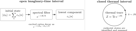
An open interval propagates specified endpoint states and can isolate the lowest-energy component present. A thermal trace identifies the endpoints at $\tau=0$ and $\tau=\beta\hbar$, producing a compact imaginary-time direction.

Construction	Operator object	Boundary data	Physical role
state propagation	$e^{-\tau H/\hbar}\lvert\psi_0\rangle$	initial state fixed	low-energy filtering
kernel	$\langle x_f\rvert e^{-\tau H/\hbar}\lvert x_i\rangle$	two endpoints fixed	heat kernel and Euclidean amplitude
matrix element	$\langle\phi\rvert e^{-\tau H/\hbar}\lvert\psi\rangle$	bra and ket fixed	spectral Laplace transform
thermal trace	$\operatorname{Tr}e^{-\beta\mathcal K}$	endpoints summed and identified	partition function
thermal correlator	$\operatorname{Tr}(e^{-\beta\mathcal K}\mathcal T_\tau\cdots)$	insertions on a circle	equilibrium fluctuations

Open propagation and a closed trace should not be interchanged. The limit $\tau\to\infty$ in an open projector is not the same operation as lowering the temperature in a normalized thermal trace, especially when degeneracies or the thermodynamic limit matter.

Thermal Trace

At temperature $T$,

$$\tau_\beta = \beta\hbar.$$

The grand partition function is

$$\mathcal Z = \operatorname{Tr} e^{-\beta\mathcal K} = \operatorname{Tr} e^{-\tau_\beta\mathcal K/\hbar}.$$

In an eigenbasis of $\mathcal K$,

$$\mathcal Z = \sum_n e^{-\beta\kappa_n}.$$

The normalized equilibrium state is

$$\rho_\beta = \frac{ e^{-\beta\mathcal K} }{ \mathcal Z }.$$

The trace closes the interval because

$$\operatorname{Tr} e^{-\beta\mathcal K} = \sum_a \langle a| e^{-\beta\mathcal K} |a\rangle.$$

The state at the final endpoint is identified with the state at the initial endpoint and then summed. In a coordinate path integral this becomes a closed path; in a coherent-state path integral it leads to periodic bosonic or antiperiodic fermionic fields.

Partition Functions owns thermodynamic derivatives of $\ln\mathcal Z$. Finite-Temperature QM Overview owns the chapter-wide representation map, Bosonic and Fermionic Matsubara Frequencies owns the allowed grids and unit conventions, Thermal Green Functions owns the ordered two-point functions and contact terms, and Matsubara Formalism Preview develops the graded Fourier series and frequency-sum workflow.

Ground-State Projection Preview

Suppose

$$H|n\rangle = E_n|n\rangle, \qquad E_0\leq E_1\leq\cdots,$$

and

$$|\psi_0\rangle = \sum_n c_n|n\rangle.$$

Then

$$e^{-\tau H/\hbar} \lvert\psi_0\rangle = e^{-\tau E_0/\hbar} \lvert\widetilde\psi(\tau)\rangle,$$

where

$$\begin{aligned} \lvert\widetilde\psi(\tau)\rangle &= c_0\lvert0\rangle \\ &\quad+ \sum_{n>0} c_n e^{-\tau(E_n-E_0)/\hbar} \lvert n\rangle. \end{aligned}$$

If $c_0\neq0$, the normalized state approaches the ground state when it is unique and separated appropriately from the rest of the spectrum.

The suppression scale for the first excited component is

$$e^{-\tau\Delta/\hbar}, \qquad \Delta=E_1-E_0.$$

Several qualifications are essential:

• if $c_0=0$, evolution cannot create ground-state overlap;
• a preserved symmetry can confine the state to a sector whose lowest state is excited globally;
• a degenerate ground space is projected as a subspace, with coefficients inherited from the initial state;
• in a gapless or continuous spectrum, convergence need not be a single exponential;
• normalization is required for a stable state interpretation;
• backward imaginary-time evolution is ill conditioned.

The canonical spectral derivation, Euclidean-kernel relation, and path-integral meaning live in Euclidean and Imaginary-Time Path Integrals. The numerical algorithm and validation protocol live in Imaginary-Time Projection.

Worked Example: Two-Level Filtering

Let

$$\begin{aligned} H &= E_0\lvert0\rangle\langle0\rvert \\ &\quad+ E_1\lvert1\rangle\langle1\rvert. \end{aligned}$$

Write the positive level spacing as $\Delta=E_1-E_0>0$, and choose

$$|\psi_0\rangle = \cos\theta\,|0\rangle +\sin\theta\,|1\rangle.$$

After imaginary time $\tau$,

$$\begin{aligned} |\psi(\tau)\rangle &= e^{-E_0\tau/\hbar} \big[ \cos\theta\,|0\rangle \\ &\qquad+ \sin\theta\, e^{-\Delta\tau/\hbar} |1\rangle \big]. \end{aligned}$$

The ground-state probability in the normalized state is

$$P_0(\tau) = \frac{ \cos^2\theta }{ \cos^2\theta + \sin^2\theta\, e^{-2\Delta\tau/\hbar} }.$$

The excited-state probability is

$$P_1(\tau) = \frac{ \sin^2\theta\, e^{-2\Delta\tau/\hbar} }{ \cos^2\theta + \sin^2\theta\, e^{-2\Delta\tau/\hbar} }.$$

Thus

$$\langle H\rangle_\tau = E_0+\Delta P_1(\tau).$$

If $\cos\theta=0$, then $P_0(\tau)=0$ for every $\tau$. Imaginary time suppresses unwanted components; it does not manufacture a missing overlap.

Normalized Imaginary-Time Flow

For projection calculations, define the normalized state

$$|\widehat\psi(\tau)\rangle = \frac{ |\psi(\tau)\rangle }{ \sqrt{ \langle\psi(\tau)|\psi(\tau)\rangle } }.$$

It obeys the nonlinear equation

$$\hbar \frac{\partial}{\partial\tau} |\widehat\psi\rangle = - \left( H-\langle H\rangle_\tau \right) |\widehat\psi\rangle.$$

For a time-independent self-adjoint Hamiltonian,

$$\frac{d}{d\tau} \langle H\rangle_\tau = -\frac{2}{\hbar} \left[ \langle H^2\rangle_\tau -\langle H\rangle_\tau^2 \right].$$

Therefore

$$\frac{d}{d\tau} \langle H\rangle_\tau = -\frac{2}{\hbar} \operatorname{Var}_\tau(H) \leq0.$$

The energy decreases until the state has support within an energy eigenspace. This is a variational descent property of normalized imaginary-time flow, not a law of physical dissipation.

Imaginary-Time Correlators and Energy Gaps

For an operator $A$, define

$$A(\tau) = e^{\tau H/\hbar} A e^{-\tau H/\hbar}.$$

At zero temperature, assume a nondegenerate ground state and consider

$$C_A(\tau) = \langle0| A(\tau) A^\dagger(0) |0\rangle.$$

Inserting energy eigenstates gives

$$C_A(\tau) = \sum_n \left| \langle n|A^\dagger|0\rangle \right|^2 e^{-(E_n-E_0)\tau/\hbar}.$$

The operator selects which excitations appear. If $\Delta_A$ is the smallest excitation energy with nonzero matrix element, then at large $\tau$

$$C_A(\tau) \sim Z_A e^{-\Delta_A\tau/\hbar},$$

provided that an isolated leading exponential exists.

Effective gap

When $C_A(\tau)>0$, define

$$\Delta_{\mathrm{eff}}(\tau) = -\hbar \frac{d}{d\tau} \ln C_A(\tau).$$

For a positive sum of discrete exponentials, this is a weighted average of excitation gaps. Its derivative is

$$\frac{ d\Delta_{\mathrm{eff}} }{ d\tau } = -\frac1\hbar \operatorname{Var}_{w(\tau)}(\Delta_n) \leq0.$$

The effective gap approaches the smallest gap carrying nonzero spectral weight. A plateau is evidence for single-exponential dominance only after finite-$\tau$, finite-size, statistical, and excited-state uncertainties are checked.

At finite temperature, the trace includes transitions among thermally occupied states and propagation around the compact interval. Correlators can contain forward and wrap-around terms. Green Functions in Many-Body QM owns the finite-temperature Lehmann and Matsubara conventions.

From Imaginary to Real Time

Writing

$$z = t-i\tau$$

gives formally

$$e^{-iz\mathcal K/\hbar} = e^{-it\mathcal K/\hbar} e^{-\tau\mathcal K/\hbar}.$$

For a lower-bounded self-adjoint generator, suitable matrix elements define analytic functions in a half-plane after an energy shift. This supplies the mathematical origin of the substitution $t=-i\tau$ in favorable cases.

Three logically distinct operations should not be conflated:

1. Spectral definition: define $e^{-\tau\mathcal K/\hbar}$ directly by functional calculus.
2. Contour rotation: deform a real-time integral into a Euclidean contour while avoiding singularities and controlling boundary terms.
3. Analytic reconstruction: infer real-frequency information from imaginary-time or Matsubara data.

The first is well defined under standard spectral assumptions. The second requires analyticity of the integrand and a valid contour deformation. The third can be severely ill conditioned when data are finite or noisy.

Time Slicing and Product Formulas

For

$$\mathcal K = T+V$$

with noncommuting pieces, one cannot generally write

$$e^{-\tau(T+V)/\hbar} = e^{-\tau T/\hbar} e^{-\tau V/\hbar}.$$

The Lie–Trotter product formula instead gives, under appropriate operator-domain assumptions,

$$\begin{aligned} e^{-\tau(T+V)/\hbar} &= \operatorname*{s-lim}_{M\to\infty} \\ &\quad \left[ e^{-\tau T/(M\hbar)} e^{-\tau V/(M\hbar)} \right]^M. \end{aligned}$$

A symmetric finite-step factorization is

$$\begin{aligned} e^{-\Delta\tau(T+V)/\hbar} &= e^{-\Delta\tau V/(2\hbar)} e^{-\Delta\tau T/\hbar} \\ &\quad\times e^{-\Delta\tau V/(2\hbar)} +O(\Delta\tau^3), \end{aligned}$$

for bounded operators or suitably controlled unbounded operators. Repeating this step over a fixed total interval produces a global error of order $\Delta\tau^2$ in the usual regular setting.

These factorizations lead to transfer matrices, worldline representations, path integrals, and projector algorithms. Operator domains and convergence mode matter in rigorous applications.

Transfer-Matrix Viewpoint

Divide the thermal interval into $M$ slices:

$$\Delta\tau = \frac{\beta\hbar}{M}.$$

Define a short-time transfer operator

$$\mathsf T = e^{-\Delta\tau\mathcal K/\hbar}.$$

Then

$$e^{-\beta\mathcal K} = \mathsf T^M,$$

and

$$\mathcal Z = \operatorname{Tr} \mathsf T^M.$$

This makes a quantum system resemble a statistical system with one additional discrete direction. The resemblance is exact at the operator level, but the resulting classical weights need not be local, real, or nonnegative.

For lattice Hamiltonians, checkerboard or Suzuki–Trotter decompositions can turn noncommuting local terms into layers of commuting gates. The continuum limit in imaginary-time spacing must be tested rather than assumed.

Numerical Uses and Failure Modes

Imaginary-time evolution appears in:

• projector methods for ground states;
• diffusion Monte Carlo;
• path-integral Monte Carlo;
• auxiliary-field methods;
• tensor-network cooling and purification;
• transfer-matrix calculations;
• extraction of masses or gaps from Euclidean correlators.

Every numerical use needs an evidence standard.

Projection calculations

Report:

• the initial overlap or symmetry sector;
• the energy shift used for numerical stability;
• the time-step rule and extrapolation;
• convergence in total imaginary time;
• normalization and orthogonalization procedure;
• comparison with exact diagonalization or a solvable limit where possible.

Thermal calculations

Report:

• system size and boundary conditions;
• number of time slices or continuous-time formulation;
• autocorrelation and equilibration checks;
• sign or phase diagnostics;
• temperature and finite-size extrapolations;
• estimator definitions and contact terms.

Spectral inference

Report:

• the imaginary-time covariance matrix;
• spectral sum rules and asymptotic moments;
• priors or regularization;
• resolution tests on synthetic data;
• uncertainty in peaks, thresholds, and continua.

Accurate imaginary-time data do not guarantee a unique real-frequency spectrum.

Common Mistakes

• Calling $\tau$ physical time. Imaginary-time evolution is nonunitary and is not a dissipative laboratory trajectory.
• Assuming Wick rotation is the definition. The semigroup is defined directly by the spectral theorem; contour rotation is a separate representation step.
• Using negative imaginary time as a stable inverse. $e^{+\tau H/\hbar}$ amplifies high-energy components and is generally unbounded.
• Forgetting the energy zero. Unnormalized norms depend on energy shifts, while normalized expectations and Boltzmann probabilities do not.
• Using $H$ instead of $H-\mu N$. Grand-canonical operator evolution is generated by $\mathcal K$.
• Assuming lower boundedness makes the thermal trace finite. Trace-class behavior also depends on spectral growth, volume, and regularization.
• Confusing an open projector with a thermal circle. Their boundary conditions and normalizations are different.
• Claiming projection reaches the global ground state without overlap. Symmetry and initial-state support can restrict the limiting sector.
• Reading every decay as one isolated gap. Degeneracies, continua, finite temperature, and multiple matrix elements can spoil a single exponential.
• Treating a plateau as proof. Fit-window, finite-size, covariance, and excited-state tests are required.
• Factorizing noncommuting exponentials exactly. Product formulas require a limit or controlled finite-step error.
• Assuming Euclidean weights are positive. Fermions, frustration, magnetic phases, and chemical potentials can produce sign or phase problems.
• Substituting $i\nu_n\to E+i0^+$ into raw data. Continuation applies to a justified analytic function, not to isolated samples.

Compact Comparison

Object	Formula	What it suppresses or encodes
real-time phase	$e^{-itE/\hbar}$	no energy-dependent norm suppression
imaginary-time factor	$e^{-\tau E/\hbar}$	high energy relative to low energy
normalized projector ratio	$e^{-\tau(E_n-E_0)/\hbar}$	excited-state contamination
Boltzmann weight	$e^{-\beta E}$	thermal occupation
thermal circumference	$\beta\hbar$	compact equilibrium time
Euclidean correlator	$\sum_n Z_n e^{-\Delta_n\tau/\hbar}$	operator-selected excitation spectrum

Cross-Links

• Thermal Density Operators defines the normalized Gibbs state.
• Partition Functions develops traces, source derivatives, and thermodynamic potentials.
• Time-Dependent Correlations contrasts real-time ordered and unordered correlators.
• Green Functions in Many-Body QM gives the particle-addition and particle-removal spectral bridge.
• Matsubara Formalism Preview continues from the thermal circle to discrete frequency sums.
• Bosonic and Fermionic Matsubara Frequencies records the periodic and antiperiodic grids, explicit-$\hbar$ units, and index conventions.
• Thermal Green Functions applies the thermal circle to graded propagators, occupations, and equal-time jumps.
• Euclidean and Imaginary-Time Path Integrals constructs the Euclidean kernel and path integral.
• Imaginary-Time Projection provides a computational benchmark.
• From Euclidean Time to Euclidean QFT extends the construction to field configurations and reconstruction questions.

References

1. E. B. Davies, Heat Kernels and Spectral Theory, Cambridge University Press (1989) – semigroups, Schrödinger heat kernels, and spectral estimates.
2. B. Simon, Functional Integration and Quantum Physics, 2nd ed., AMS Chelsea (2005) – Feynman–Kac methods and functional integration for nonrelativistic quantum mechanics.
3. H. F. Trotter, “On the Product of Semi-Groups of Operators”, Proceedings of the American Mathematical Society 10, 545–551 (1959) – product formula underlying time slicing.
4. R. P. Feynman, “Atomic Theory of the $\lambda$ Transition in Helium”, Physical Review 91, 1291–1301 (1953) – early path-integral treatment of quantum statistical mechanics.
5. T. Matsubara, “A New Approach to Quantum-Statistical Mechanics”, Progress of Theoretical Physics 14, 351–378 (1955) – imaginary-time many-body formalism.
6. D. M. Ceperley, “Path Integrals in the Theory of Condensed Helium”, Reviews of Modern Physics 67, 279–355 (1995) – path-integral Monte Carlo and finite-temperature many-body applications.
7. A. L. Fetter and J. D. Walecka, Quantum Theory of Many-Particle Systems, Dover (2003 reprint of the 1971 edition) – equilibrium propagators, imaginary time, and spectral representations.
8. P. Coleman, Introduction to Many-Body Physics, Cambridge University Press (2015) – modern operator and finite-temperature many-body treatment.

Exercises

1. Semigroup norm

Let $\mathcal K$ be self-adjoint with

$$\inf\operatorname{spec}\mathcal K = \kappa_{\min}.$$

Use the spectral theorem to show

$$\left\| e^{-\tau\mathcal K/\hbar} \right\| = e^{-\tau\kappa_{\min}/\hbar}.$$

What changes after shifting $\mathcal K$ by $-\kappa_{\min}I$?

Solution

For a bounded Borel function $f$ of a self-adjoint operator,

$$\|f(\mathcal K)\| = \sup_{\kappa\in\operatorname{spec}\mathcal K} |f(\kappa)|.$$

With

$$f(\kappa) = e^{-\tau\kappa/\hbar}$$

and $\tau\geq0$, the largest value occurs at the lower spectral edge. Hence

$$\left\| e^{-\tau\mathcal K/\hbar} \right\| = e^{-\tau\kappa_{\min}/\hbar}.$$

For

$$\widetilde{\mathcal K} = \mathcal K-\kappa_{\min}I,$$

the lower edge is zero, so

$$\left\| e^{-\tau\widetilde{\mathcal K}/\hbar} \right\| = 1.$$

The shift multiplies the unnormalized propagator by $e^{+\tau\kappa_{\min}/\hbar}$ but leaves normalized state ratios unchanged.

2. Energy descent

Suppose a normalized state obeys

$$\hbar \partial_\tau|\psi\rangle = - \left( H-\langle H\rangle \right) |\psi\rangle.$$

Derive

$$\partial_\tau\langle H\rangle = -\frac{2}{\hbar} \operatorname{Var}(H).$$

Solution

For time-independent $H$,

$$\partial_\tau\langle H\rangle = \langle\partial_\tau\psi|H|\psi\rangle + \langle\psi|H|\partial_\tau\psi\rangle.$$

Insert the evolution equation and its adjoint:

$$\begin{aligned} \partial_\tau\langle H\rangle &= -\frac1\hbar \langle (H-\langle H\rangle)H \rangle \\ &\quad -\frac1\hbar \langle H(H-\langle H\rangle) \rangle \\ &= -\frac{2}{\hbar} \left( \langle H^2\rangle -\langle H\rangle^2 \right). \end{aligned}$$

The variance is nonnegative, so normalized imaginary-time flow cannot increase the energy expectation.

3. Projection time for a two-level state

For the two-level example, find a condition on $\tau$ that guarantees

$$P_1(\tau) \leq \varepsilon,$$

where $0\lt\varepsilon\lt1$ and both initial amplitudes are nonzero.

Solution

Write

$$r = \tan^2\theta\, e^{-2\Delta\tau/\hbar}.$$

Then

$$P_1 = \frac{r}{1+r}.$$

The condition $P_1\leq\varepsilon$ is equivalent to

$$r \leq \frac{\varepsilon}{1-\varepsilon}.$$

Therefore it is sufficient that

$$\tau \geq \frac{\hbar}{2\Delta} \ln \left[ \tan^2\theta \frac{1-\varepsilon}{\varepsilon} \right].$$

If the logarithm is negative, the requested tolerance already holds at $\tau=0$, so the minimal nonnegative projection time is zero.

4. Free heat kernel

Show that the $d$-dimensional free kernel satisfies

$$\partial_\tau K_{\mathrm E} = \frac{\hbar}{2m} \nabla^2 K_{\mathrm E}$$

and approaches a delta distribution as $\tau\to0^+$.

Solution

Write

$$K_{\mathrm E}(\mathbf r,\tau) = \left( \frac{m}{2\pi\hbar\tau} \right)^{d/2} \exp \left( -\frac{m\mathbf r^2}{2\hbar\tau} \right).$$

Direct differentiation gives

$$\frac{ \partial_\tau K_{\mathrm E} }{ K_{\mathrm E} } = -\frac{d}{2\tau} + \frac{ m\mathbf r^2 }{ 2\hbar\tau^2 }.$$

The Laplacian gives

$$\frac{ \nabla^2 K_{\mathrm E} }{ K_{\mathrm E} } = -\frac{ dm }{ \hbar\tau } + \frac{ m^2\mathbf r^2 }{ \hbar^2\tau^2 }.$$

Multiplying by $\hbar/(2m)$ reproduces the time derivative. The Gaussian is normalized for every $\tau>0$, and its width is of order

$$\sqrt{ \frac{\hbar\tau}{m} }.$$

As $\tau\to0^+$, the width vanishes while the integral remains one. Hence the kernel converges to $\delta^{(d)}(\mathbf r)$ in the distributional sense.

5. Energy shifts in a thermal trace

Let

$$H' = H+C I.$$

Show how $Z$, $\rho_\beta$, and a normalized thermal expectation change.

Solution

The shifted partition function is

$$\begin{aligned} Z' &= \operatorname{Tr} e^{-\beta(H+CI)} \\ &= e^{-\beta C}Z. \end{aligned}$$

The shifted density operator is

$$\rho_\beta' = \frac{ e^{-\beta C}e^{-\beta H} }{ e^{-\beta C}Z } = \rho_\beta.$$

Therefore every normalized expectation

$$\operatorname{Tr} (\rho_\beta A)$$

is unchanged. The free energy shifts by $C$, as expected for a change of energy zero.

6. Effective-gap monotonicity

Let

$$C(\tau) = \sum_n w_n e^{-\Delta_n\tau/\hbar}, \qquad w_n>0.$$

Show that

$$\Delta_{\mathrm{eff}} = -\hbar\partial_\tau\ln C$$

is a weighted mean of the $\Delta_n$ and decreases monotonically with $\tau$.

Solution

Define normalized $\tau$-dependent weights

$$p_n(\tau) = \frac{ w_n e^{-\Delta_n\tau/\hbar} }{ C(\tau) }.$$

Then

$$\sum_n p_n=1$$

and

$$\Delta_{\mathrm{eff}} = \sum_n p_n\Delta_n.$$

Differentiating the weights gives

$$\partial_\tau p_n = -\frac1\hbar p_n \left( \Delta_n-\Delta_{\mathrm{eff}} \right).$$

Therefore

$$\partial_\tau\Delta_{\mathrm{eff}} = \sum_n \Delta_n \partial_\tau p_n.$$

Substitution yields

$$\begin{aligned} \partial_\tau\Delta_{\mathrm{eff}} &= -\frac1\hbar \Bigg[ \sum_n p_n\Delta_n^2 \\ &\qquad- \left( \sum_n p_n\Delta_n \right)^2 \Bigg]. \end{aligned}$$

Equivalently,

$$\partial_\tau\Delta_{\mathrm{eff}} = -\frac1\hbar \operatorname{Var}_{p(\tau)}(\Delta) \leq0.$$

Equality holds only when the contributing gaps are all equal. At large $\tau$, the smallest gap with nonzero weight dominates.

7. Grand-canonical operator evolution

For one fermionic mode,

$$H = \epsilon c^\dagger c, \qquad N = c^\dagger c,$$

derive $c(\tau)$ using $\mathcal K=H-\mu N$. What incorrect factor would result from evolving with $H$ alone?

Solution

The ensemble generator is

$$\mathcal K = (\epsilon-\mu)c^\dagger c = \xi c^\dagger c.$$

Since

$$[c^\dagger c,c] = -c,$$

the imaginary-time Heisenberg equation gives

$$\hbar\partial_\tau c(\tau) = -\xi c(\tau).$$

Hence

$$c(\tau) = e^{-(\epsilon-\mu)\tau/\hbar}c.$$

Using $H$ alone would give $e^{-\epsilon\tau/\hbar}$ and would miss the chemical-potential shift that aligns the propagator with grand-canonical thermal weights.