Euclidean Time and Imaginary-Time Action

Euclidean time turns selected quantum amplitudes into damping problems. For a time-independent Hamiltonian, the basic operator is

$$e^{-\hat H T/\hbar}, \qquad T\gt0,$$

and for a particle with real-time Lagrangian

$$L_M = \frac{m}{2}\dot x^2 - V(x),$$

the corresponding Euclidean action is

$$S_E[x] = \int d\tau \left[ \frac{m}{2}(x')^2 + V(x) \right].$$

Here a dot denotes $d/dt$, a prime denotes $d/d\tau$, and the contour convention is $t=-i\tau$. The positive sign of the Euclidean kinetic term is essential.

This page owns the tunneling-oriented Euclidean mechanics: sign conventions, background subtraction, boundary terms, conserved Euclidean energy, fixed-time versus fixed-energy exponents, and reliability checks. Euclidean and Imaginary-Time Path Integrals owns the time-sliced Euclidean kernel, thermal trace, and exact harmonic-oscillator kernel. Instantons in Quantum Mechanics owns the explicit saddle construction and its use in tunneling splittings.

The Rotation t → −iτ

Real-time evolution is generated by

$$U(t) = e^{-i\hat Ht/\hbar}.$$

At the imaginary-time endpoint $t=-iT$,

$$U(-iT) = e^{-\hat H T/\hbar}.$$

A useful way to picture the continuation is to rotate the time contour continuously,

$$t = e^{-i\theta}s, \qquad 0\leq\theta\leq\frac{\pi}{2}, \qquad s\geq0.$$

The Lorentzian contour is $\theta=0$; the Euclidean contour is $\theta=\pi/2$. The word Wick rotation refers to this contour deformation, not merely to replacing one symbol by another.

If $\hat H$ is self-adjoint and bounded below by $E_0$, the operator $e^{-\hat H T/\hbar}$ is well defined for $T\gt0$, with

$$\left\| e^{-\hat H T/\hbar} \right\| = e^{-E_0T/\hbar}.$$

The overall norm can grow when $E_0\lt0$, but high-energy components are still damped relative to low-energy components. Shifting $\hat H$ by a constant changes only the common normalization factor.

Three statements that must be separated

The following statements are related, but they are not interchangeable:

1. Operator continuation: define the semigroup $e^{-\hat H T/\hbar}$ by spectral calculus.
2. Kernel continuation: analytically continue a real-time kernel in a domain free of obstructing singularities.
3. Path-integral deformation: deform an integration cycle so that $e^{iS_M/\hbar}$ becomes a convergent or asymptotic Euclidean integral.

The first can be meaningful even when no simple real-time path integral is available. The third requires information about integration contours and singularities that is not contained in the symbolic substitution $t=-i\tau$.

From Lorentzian to Euclidean Action

Start with

$$S_M[x] = \int dt \left[ \frac{m}{2}\dot x^2 - V(x) \right].$$

Under

$$t=-i\tau, \qquad dt=-i\,d\tau, \qquad \dot x=i x',$$

the action becomes

$$\begin{aligned} S_M[x] &= \int(-i\,d\tau) \left[ -\frac{m}{2}(x')^2 - V(x) \right] \\ &= i \int d\tau \left[ \frac{m}{2}(x')^2 + V(x) \right] \\ &= iS_E[x]. \end{aligned}$$

Therefore

$$\frac{i}{\hbar}S_M = -\frac{1}{\hbar}S_E, \qquad e^{iS_M/\hbar} \longrightarrow e^{-S_E/\hbar}.$$

For several coordinates $q^a$ with a positive configuration-space metric $G_{ab}(q)$,

$$L_M = \frac12 G_{ab}(q)\dot q^a\dot q^b - V(q)$$

continues to

$$S_E[q] = \int d\tau \left[ \frac12 G_{ab}(q)q^{\prime a}q^{\prime b} + V(q) \right].$$

Positivity of the kinetic form matters. A nonstandard kinetic term, constrained system, or momentum-dependent interaction requires its own continuation rather than this template.

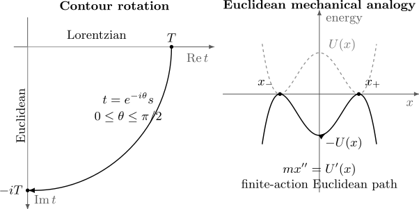
The time contour rotates from the positive real axis to $t=-iT$. The Euclidean equation of motion is equivalent to ordinary motion in the inverted potential $-U(x)$, but the Euclidean saddle is not a hidden real-time trajectory.

The sign audit

Three quick checks catch most sign errors:

• The free-particle Euclidean action must contain $+m(x')^2/2$.
• A stable harmonic potential $V=m\omega^2x^2/2$ must contribute $+m\omega^2x^2/2$.
• Varying $S_E$ must give $mx''=V'(x)$, which is motion in the inverted potential $-V$.

The potential is inverted in the equation-of-motion analogy, not in $S_E$. Writing $S_E$ with $-V$ would destroy the damping structure of the stable oscillator.

Potential shifts and background subtraction

Suppose a reference configuration $x_{\mathrm{ref}}$ has energy

$$V_{\mathrm{ref}} = V(x_{\mathrm{ref}}).$$

Define

$$U(x) = V(x)-V_{\mathrm{ref}}.$$

Then

$$S_E[x] = V_{\mathrm{ref}}T + \int d\tau \left[ \frac{m}{2}(x')^2 + U(x) \right].$$

The constant $V_{\mathrm{ref}}T$ matters for an absolute kernel, but it cancels from normalized ratios and from a saddle action measured relative to the reference background. For tunneling on an infinite Euclidean interval, the finite quantity is normally

$$\begin{aligned} B[x] &\equiv S_E[x]-S_E[x_{\mathrm{ref}}] \\ &= \int_{-\infty}^{\infty} d\tau \left[ \frac{m}{2}(x')^2 + U(x) \right]. \end{aligned}$$

Failing to subtract the background can turn a finite tunneling exponent into an irrelevant infinite vacuum contribution.

Velocity-linear terms

Euclidean actions need not be real. For example, in several dimensions,

$$L_M = \frac{m}{2}\dot{\mathbf x}^{\,2} + q\mathbf A(\mathbf x)\cdot\dot{\mathbf x} - V(\mathbf x)$$

gives

$$\begin{aligned} S_E &= \int d\tau \left[ \frac{m}{2}(\mathbf x')^2 + V(\mathbf x) \right] \\ &\quad- iq\int d\tau\, \mathbf A(\mathbf x)\cdot\mathbf x'. \end{aligned}$$

The magnetic line integral becomes an imaginary part of $S_E$. The real part can still damp paths, while the imaginary part carries phase information. Thus “Euclidean” does not always mean “positive real weight.”

Imaginary-Time Schrödinger Evolution

The real-time Schrödinger equation is

$$i\hbar \frac{\partial}{\partial t} \vert\psi(t)\rangle = \hat H\vert\psi(t)\rangle.$$

Since $t=-i\tau$ implies $\partial_t=i\partial_\tau$, imaginary-time evolution obeys

$$\hbar \frac{\partial}{\partial\tau} \vert\psi(\tau)\rangle = -\hat H\vert\psi(\tau)\rangle.$$

For

$$\hat H = -\frac{\hbar^2}{2m} \frac{\partial^2}{\partial x^2} + V(x),$$

the wavefunction satisfies the diffusion-reaction equation

$$\hbar \frac{\partial\psi}{\partial\tau} = \frac{\hbar^2}{2m} \frac{\partial^2\psi}{\partial x^2} - V(x)\psi.$$

This equation is parabolic rather than unitary. It smooths short-wavelength structure while damping regions with positive potential relative to the chosen energy reference. The connection to Wiener measure and diffusion is formalized, under suitable hypotheses, by the Feynman–Kac formula.

Normalized imaginary-time flow

The unnormalized norm is not conserved. If the state is normalized after each Euclidean-time step, write it as $\vert\phi(\tau)\rangle$. Its evolution is

$$\hbar \frac{\partial}{\partial\tau} \vert\phi\rangle = - \left( \hat H-\langle\hat H\rangle_\phi \right) \vert\phi\rangle.$$

For a time-independent Hermitian Hamiltonian,

$$\frac{d}{d\tau} \langle\hat H\rangle_\phi = - \frac{2}{\hbar} \left[ \langle\hat H^2\rangle_\phi - \langle\hat H\rangle_\phi^2 \right] \leq0.$$

Normalized imaginary-time evolution therefore lowers the energy expectation monotonically, stopping only when the state has support inside an energy eigenspace. This is a computational descent principle, not physical dissipative time evolution.

Ground-State Projection and Its Scales

Let

$$\hat H\vert n\rangle = E_n\vert n\rangle, \qquad E_0\leq E_1\leq\cdots,$$

and

$$\vert\psi\rangle = \sum_n c_n\vert n\rangle.$$

Then

$$\begin{aligned} e^{-\hat H T/\hbar}\vert\psi\rangle &= e^{-E_0T/\hbar} \Bigg[ c_0\vert0\rangle \\ &\quad+ \sum_{n\gt0} c_ne^{-(E_n-E_0)T/\hbar} \vert n\rangle \Bigg]. \end{aligned}$$

If $c_0\ne0$ and the ground state is nondegenerate, normalization leaves $\vert0\rangle$ as $T\to\infty$. If the ground space is degenerate, the limit is the normalized projection into that subspace.

The relative contamination of level $n$ is

$$r_n(T) = \frac{c_n}{c_0} e^{-(E_n-E_0)T/\hbar}.$$

To make the first excited contribution smaller than a target $\delta$, it is sufficient that

$$T \geq \frac{\hbar}{E_1-E_0} \log\left( \frac{|c_1|} {\delta|c_0|} \right),$$

when the logarithm is positive. Projection time is controlled by the gap and by trial-state overlap, not by a universal number of time steps.

The double-well hierarchy

In a deep symmetric double well, the tunneling splitting $\Delta_{\mathrm{tun}}$ can be exponentially smaller than the intrawell excitation scale $\hbar\omega$. Two Euclidean-time requirements are then parametrically different:

$$T \gg \frac{1}{\omega}$$

suppresses higher intrawell excitations, whereas

$$T \gg \frac{\hbar}{\Delta_{\mathrm{tun}}}$$

is needed to isolate one parity eigenstate from the low-energy doublet.

The intermediate window

$$\frac{1}{\omega} \ll T \ll \frac{\hbar}{\Delta_{\mathrm{tun}}}$$

projects efficiently onto the two-dimensional low-energy subspace without resolving its exponentially small splitting. This distinction is central in numerical tunneling calculations.

Tunneling Splittings turns this hierarchy into a practical Euclidean-kernel estimator for the doublet gap.

Extracting the ground energy

For boundary states with nonzero ground-state overlap, define

$$Z_{\chi\psi}(T) = \langle\chi\vert e^{-\hat H T/\hbar} \vert\psi\rangle.$$

At large $T$,

$$\begin{aligned} E_0 &= - \hbar \frac{d}{dT} \log Z_{\chi\psi}(T) \\ &\quad+ O\left( (E_1-E_0) e^{-(E_1-E_0)T/\hbar} \right), \end{aligned}$$

provided the leading coefficient does not vanish through symmetry or cancellation. Ratios at nearby $T$ values are often more stable than the exponentially small kernel itself.

Varying the Euclidean Action

For the background-subtracted action

$$B[x] = \int_{\tau_i}^{\tau_f} d\tau \left[ \frac{m}{2}(x')^2 + U(x) \right],$$

the first variation is

$$\begin{aligned} \delta B &= \left[ mx'\delta x \right]_{\tau_i}^{\tau_f} \\ &\quad+ \int_{\tau_i}^{\tau_f} d\tau \left[ -mx'' + U'(x) \right]\delta x. \end{aligned}$$

For fixed endpoints, $\delta x(\tau_i)=\delta x(\tau_f)=0$, so stationarity gives

$$mx'' = U'(x) = V'(x).$$

This is Newton’s equation in the inverted potential $-U(x)$:

$$mx'' = - \frac{d}{dx} \left[ -U(x) \right].$$

The analogy helps solve the boundary-value problem. It does not mean that the quantum particle follows $x(\tau)$ in real time.

Boundary terms are physical data

Different observables eliminate or modify the endpoint term in different ways:

Euclidean object	Endpoint data
Fixed-endpoint kernel	$\delta x(\tau_i)=\delta x(\tau_f)=0$
Thermal trace	$x(\tau_f)=x(\tau_i)$ and matching Euclidean momentum
Instanton	endpoints approach distinct degenerate minima as $\tau\to\pm\infty$
Bounce	both ends approach the same metastable minimum
Wavefunction-weighted endpoint	boundary variation is balanced by the logarithmic derivative of the endpoint wavefunction

Choosing a saddle before choosing these data reverses the logic. The boundary conditions define the observable; only then can one identify the relevant stationary configurations.

Conserved Euclidean energy

If $U$ has no explicit $\tau$ dependence, the Euclidean Noether energy is

$$\mathcal E_E = x' \frac{\partial L_E}{\partial x'} - L_E = \frac{m}{2}(x')^2 - U(x).$$

It is constant along a saddle:

$$\frac{d\mathcal E_E}{d\tau} = 0.$$

For a finite-action path approaching a reference minimum with

$$U(x_{\mathrm{ref}})=0, \qquad x'\to0,$$

one has $\mathcal E_E=0$. Therefore

$$\frac{m}{2}(x')^2 = U(x).$$

For a monotone path between degenerate minima,

$$\begin{aligned} B &= \int d\tau \left[ \frac{m}{2}(x')^2 + U(x) \right] \\ &= \int_{x_-}^{x_+} dx\, \sqrt{2mU(x)}. \end{aligned}$$

This action identity is the bridge to the WKB forbidden-region exponent. The explicit instanton profile, collective coordinate, and determinant belong to Instantons in Quantum Mechanics.

Exponential approach to a minimum

Near a nondegenerate minimum $x_\star$, write $x=x_\star+\eta$ and

$$U(x) = \frac{m\omega_\star^2}{2}\eta^2 + O(\eta^3).$$

The linearized Euclidean equation is

$$\eta'' = \omega_\star^2\eta.$$

A finite-action tail must select the decaying branch,

$$\eta(\tau) \propto e^{-\omega_\star|\tau-\tau_0|}.$$

This tail supplies practical boundary data for numerical shooting and explains why truncation errors on a finite Euclidean interval are exponentially small in the endpoint distance from the saddle center.

Fixed-Time and Fixed-Energy Exponents

A common source of factor and sign errors is to confuse a kernel at fixed Euclidean duration with a tunneling amplitude at fixed energy.

At fixed $T$, a saddle contributes schematically

$$K_E(T) \sim A(T) e^{-S_E(T)/\hbar}.$$

An energy-resolved Green function can be represented, for suitable $E$, by

$$G_E(E;x_f,x_i) \equiv \langle x_f\vert (\hat H-E)^{-1} \vert x_i\rangle.$$

Its Euclidean representation is

$$\begin{aligned} G_E(E;x_f,x_i) &= \frac{1}{\hbar} \int_0^\infty dT \\ &\quad\times e^{ET/\hbar} K_E(x_f,T;x_i,0). \end{aligned}$$

Its semiclassical exponent is therefore

$$S_E(T)-ET.$$

Stationarity with respect to $T$ selects a trajectory with Euclidean energy

$$\mathcal E_E = -E,$$

so

$$\frac{m}{2}(x')^2 = V(x)-E.$$

The fixed-energy abbreviated action is the Legendre transform

$$W(E) = S_E(T)-ET.$$

Between turning points $x_1(E)$ and $x_2(E)$,

$$\begin{aligned} W(E) &= \int d\tau \left[ \frac{m}{2}(x')^2 + V(x)-E \right] \\ &= \int_{x_1(E)}^{x_2(E)} dx\, \sqrt{2m[V(x)-E]}. \end{aligned}$$

Thus the forbidden-region wavefunction amplitude carries

$$e^{-W(E)/\hbar},$$

while a leading one-dimensional transmission probability carries

$$e^{-2W(E)/\hbar}.$$

The factor of two distinguishes an amplitude exponent from a probability exponent. Barrier Penetration and Tunneling owns the connection formulas and transmission calculation.

A Calculation-Ready Workflow

For a Euclidean tunneling calculation:

1. Name the observable. Decide whether the target is a kernel, splitting, transition amplitude, resonance width, decay rate, or thermal trace.
2. State the limiting family. Identify the dimensionless small parameter, often $\hbar/S_\star$ or a weak coupling that makes $S_\star/\hbar$ large.
3. Fix the boundary data. Specify endpoints, asymptotic vacua, periodicity, or outgoing-state information before solving an equation.
4. Choose the energy reference. Subtract the appropriate vacuum or false-vacuum background.
5. Derive the Euclidean action. Continue every term, including velocity-linear and explicitly time-dependent terms.
6. Audit the signs. Check the free particle, a stable quadratic fluctuation, and the inverted-potential equation.
7. Solve the saddle problem. Use the second-order equation or a justified first integral.
8. Evaluate the action independently. Compare direct quadrature in $\tau$ with the first-integral expression in configuration space.
9. Inspect fluctuations. Count zero modes and negative modes before interpreting the saddle.
10. State the claimed accuracy. Distinguish the exponent, one-loop prefactor, and multi-saddle sector sum.
11. Validate. Compare with WKB, exact diagonalization, a grid calculation, or a limiting case.

Numerical diagnostics

A robust numerical implementation should:

• nondimensionalize the coordinate, Euclidean time, and action;
• monitor the conserved $\mathcal E_E$ along the trajectory;
• place finite-interval endpoints several tail lengths $1/\omega_\star$ from the event center;
• subtract the reference action before taking a large-$T$ limit;
• vary the interval and mesh independently;
• evaluate the action both from $m(x')^2/2+U$ and from the first integral when available;
• separate an exact translation zero mode from a small numerical eigenvalue.

An accurate trajectory does not guarantee an accurate exponential if the action is obtained by subtracting two large, nearly equal quantities. Background subtraction should be built into the integrand whenever possible.

When Wick Rotation Is Not Automatic

The formal continuation can fail or become incomplete for several reasons.

Singularities and contour obstructions

A kernel or integrand may have poles, branch cuts, or essential growth in the region swept out by the contour. Deforming across a singularity changes the answer by residues or discontinuities. The correct real-time boundary prescription must be carried through the deformation.

Hamiltonians not bounded below

If the spectrum extends to $-\infty$, $e^{-\hat H T/\hbar}$ amplifies increasingly negative energies and need not define a bounded semigroup. A Euclidean kinetic term that looks positive does not repair an unstable quantum Hamiltonian.

Complex Euclidean actions

Magnetic terms, Berry phases, chemical potentials, real-time sources, and complex saddles can make $S_E$ complex. The integral then retains a phase problem and may require a deformed integration cycle.

Explicit time dependence

For $V(x,t)$, the continuation produces $V(x,-i\tau)$. Analyticity and the chosen contour become part of the problem, and the Euclidean action may be complex or nonlocal.

Real-time observables

Euclidean correlators can encode spectra, but recovering retarded response, transport, or late-time oscillations requires analytic continuation with the correct boundary values. Numerically, that inverse problem can be severely ill-conditioned.

Metastability

A metastable state is not an exact normalizable energy eigenstate with a real discrete eigenvalue. Its decay rate is extracted through analytic continuation, resonance boundary conditions, and the negative mode of a bounce. False Vacuum Decay in Quantum Mechanics develops the corresponding resonance width, survival probability, and nonexponential time regimes. Simple ground-state projection does not by itself produce a decay law.

Open and non-Hermitian dynamics

A Lindblad generator or non-Hermitian effective Hamiltonian does not generally become an equilibrium Euclidean action under $t=-i\tau$. Its spectrum, left and right eigenvectors, and contour structure must be treated on their own terms.

Bridge to Euclidean QFT

For a real scalar field in $d$ spatial dimensions,

$$\begin{aligned} S_M[\phi] &= \int dt\,d^d x\, \mathcal L_M, \\ S_E[\phi] &= \int d\tau\,d^d x\, \mathcal L_E. \end{aligned}$$

The Lorentzian and Euclidean densities are

$$\begin{aligned} \mathcal L_M &= \frac12(\partial_t\phi)^2 - \frac12(\boldsymbol\nabla\phi)^2 \\ &\quad- V(\phi), \\ \mathcal L_E &= \frac12(\partial_\tau\phi)^2 + \frac12(\boldsymbol\nabla\phi)^2 \\ &\quad+ V(\phi). \end{aligned}$$

The Euclidean field equation is

$$- \partial_\tau^2\phi - \boldsymbol\nabla^2\phi + V'(\phi) = 0.$$

Quantum mechanics is the $0+1$-dimensional case: there is no spatial gradient term, and the field configuration on a time slice reduces to one or finitely many coordinates. In field theory, the saddle is a function of Euclidean spacetime, its finite-action boundary conditions are imposed at spatial and temporal infinity, and fluctuations are differential operators in $d+1$ dimensions.

The translation is structural, not automatic. Gauge fixing, topology, renormalization, fermion zero modes, reflection positivity, and Lorentzian reconstruction add genuinely field-theoretic issues. From Euclidean Time to Euclidean QFT owns the vacuum-functional, thermal-circle, Matsubara, and reconstruction dictionary. Bridge to QFT Instantons focuses on how finite-action quantum-mechanical saddles generalize to fields.

Common Mistakes

• Replacing $t$ by $-i\tau$ without transforming $dt$ and $\dot x$.
• Putting $-V$ in the Euclidean action because the mechanical analogy uses an inverted potential.
• Treating the Euclidean saddle as a real-time trajectory under a barrier.
• Forgetting to subtract the vacuum background on an infinite Euclidean interval.
• Calling $e^{-S_E/\hbar}$ a probability density without a measure, normalization, and boundary conditions.
• Confusing a fixed-time action $S_E(T)$ with the fixed-energy exponent $W(E)=S_E-ET$.
• Using the amplitude exponent for a transmission probability and missing a factor of two.
• Assuming positive Euclidean kinetic energy guarantees that the full action is real and bounded below.
• Projecting onto the wrong symmetry sector because the trial state has zero overlap with the desired state.
• Interpreting normalized imaginary-time evolution as physical dissipation.
• Choosing an instanton or bounce before specifying which observable and endpoint conditions are required.
• Ignoring zero and negative modes when converting a saddle action into a physical prefactor.

Exercises

1. Derive both Euclidean signs

For

$$L_M = \frac{m}{2}\dot x^2 - V(x),$$

use $t=-i\tau$ to derive the Euclidean action and the imaginary-time Schrödinger equation. Explain why the kinetic term in $S_E$ and the diffusion term in the Schrödinger equation have the signs shown on this page.

Solution

The derivatives transform as

$$dt=-i\,d\tau, \qquad \dot x = \frac{dx}{dt} = ix'.$$

Therefore

$$\begin{aligned} S_M &= \int(-i\,d\tau) \left[ -\frac{m}{2}(x')^2 - V \right] \\ &= i \int d\tau \left[ \frac{m}{2}(x')^2 + V \right] = iS_E. \end{aligned}$$

Hence $iS_M/\hbar=-S_E/\hbar$, so convergence around a stable quadratic configuration requires the positive Euclidean kinetic term.

Also $\partial_t=i\partial_\tau$. Substituting into

$$i\hbar\partial_t\psi = \left[ -\frac{\hbar^2}{2m}\partial_x^2 + V \right]\psi$$

gives

$$\hbar\partial_\tau\psi = \frac{\hbar^2}{2m}\partial_x^2\psi - V\psi.$$

The positive coefficient of $\partial_x^2$ is the diffusion sign. It is consistent with Gaussian smoothing by the free Euclidean kernel.

2. Prove monotonic energy descent

Let a normalized state obey

$$\hbar\partial_\tau\vert\phi\rangle = - \left( \hat H-\langle\hat H\rangle \right) \vert\phi\rangle.$$

Show that its energy expectation is nonincreasing and identify the condition for equality.

Solution

For time-independent Hermitian $\hat H$,

$$\begin{aligned} \frac{d}{d\tau}\langle\hat H\rangle &= \langle\partial_\tau\phi\vert \hat H \vert\phi\rangle + \langle\phi\vert \hat H \vert\partial_\tau\phi\rangle \\ &= - \frac{2}{\hbar} \langle \hat H \left( \hat H-\langle\hat H\rangle \right) \rangle \\ &= - \frac{2}{\hbar} \left( \langle\hat H^2\rangle - \langle\hat H\rangle^2 \right). \end{aligned}$$

The bracket is the energy variance, so it is nonnegative. Equality holds exactly when the state has zero energy variance, meaning that its support lies within one energy eigenspace. Degeneracy allows any superposition inside that eigenspace.

3. Resolve a doublet, or only its subspace

A deep double well has tunneling splitting $\Delta_{\mathrm{tun}}$ and an intrawell gap approximately $\hbar\omega$, with $\Delta_{\mathrm{tun}}\ll\hbar\omega$.

1. Give a Euclidean-time regime that suppresses intrawell excitations but does not resolve the doublet.
2. Give the regime needed to isolate the unique parity ground state.
3. Explain what happens if the trial state has odd parity.

Solution

Intrawell excitations are suppressed by factors of order $e^{-\omega T}$, while the unwanted partner in the doublet is suppressed only by

$$e^{-\Delta_{\mathrm{tun}}T/\hbar}.$$

Therefore

$$\frac{1}{\omega} \ll T \ll \frac{\hbar}{\Delta_{\mathrm{tun}}}$$

projects onto the low-energy doublet without selecting one member. Isolating the even ground state requires

$$T \gg \frac{\hbar}{\Delta_{\mathrm{tun}}}.$$

If the Hamiltonian preserves parity and the trial state is purely odd, its overlap with the even ground state vanishes. Imaginary-time evolution preserves the odd sector and projects onto the lowest odd state instead.

4. Obtain the finite-action first integral

Let $U(x_\pm)=0$ at two degenerate minima. A monotone Euclidean saddle obeys

$$mx'' = U'(x)$$

and approaches $x_\pm$ with $x'\to0$ as $\tau\to\pm\infty$. Derive its first integral and reduce the background-subtracted action to a configuration-space integral.

Solution

Multiply the equation by $x'$:

$$mx''x' = U'(x)x'.$$

Both sides are total derivatives, so

$$\frac{d}{d\tau} \left[ \frac{m}{2}(x')^2 - U(x) \right] = 0.$$

The endpoint conditions set the constant to zero:

$$\frac{m}{2}(x')^2 = U(x).$$

For the increasing branch,

$$x' = \sqrt{\frac{2U(x)}{m}}.$$

Then

$$\begin{aligned} B &= \int d\tau \left[ \frac{m}{2}(x')^2 + U \right] \\ &= \int d\tau\,2U \\ &= \int_{x_-}^{x_+} dx\, \sqrt{2mU(x)}. \end{aligned}$$

The decreasing branch has the same positive action after reversing the integration limits and the sign of $x'$.

5. Recover the WKB action from fixed energy

Starting from a fixed-time Euclidean saddle with action $S_E(T)$, explain why an energy-resolved amplitude uses $S_E(T)-ET$. Show that its stationary trajectory satisfies

$$\frac{m}{2}(x')^2 = V(x)-E$$

and derive the forbidden-region action $W(E)$.

Solution

The resolvent representation contains

$$\int_0^\infty dT\, \exp\left[ - \frac{S_E(T)-ET}{\hbar} \right].$$

Varying $T$ gives

$$\frac{\partial S_E}{\partial T} = E.$$

Hamilton–Jacobi theory gives

$$\frac{\partial S_E}{\partial T} = -\mathcal E_E,$$

so $\mathcal E_E=-E$. Since

$$\mathcal E_E = \frac{m}{2}(x')^2 - V(x),$$

one obtains

$$\frac{m}{2}(x')^2 = V(x)-E.$$

Finally,

$$\begin{aligned} W(E) &= S_E-ET \\ &= \int d\tau \left[ \frac{m}{2}(x')^2 + V-E \right] \\ &= \int_{x_1}^{x_2} dx\, \sqrt{2m[V(x)-E]}. \end{aligned}$$

This is the WKB action for the forbidden interval. It controls an amplitude as $e^{-W/\hbar}$ and a leading transmission probability as $e^{-2W/\hbar}$.

6. Continue a magnetic line term

For a particle in several dimensions with

$$L_M = \frac{m}{2}\dot{\mathbf x}^{\,2} + q\mathbf A(\mathbf x)\cdot\dot{\mathbf x} - V(\mathbf x),$$

derive $S_E$ under $t=-i\tau$. Why does the Euclidean weight remain complex even if the kinetic and potential terms are nonnegative?

Solution

The kinetic and potential terms give

$$i \int d\tau \left[ \frac{m}{2}(\mathbf x')^2 + V \right]$$

in $S_M$. The velocity-linear term is a line integral:

$$\begin{aligned} \int dt\, q\mathbf A\cdot\dot{\mathbf x} &= q\int\mathbf A\cdot d\mathbf x \\ &= q\int d\tau\, \mathbf A\cdot\mathbf x'. \end{aligned}$$

Thus

$$S_M = iS_{E,0} + q\int d\tau\, \mathbf A\cdot\mathbf x',$$

and $iS_M=-S_E$ implies

$$S_E = \int d\tau \left[ \frac{m}{2}(\mathbf x')^2 + V - iq\mathbf A\cdot\mathbf x' \right].$$

The Euclidean weight is

$$e^{-S_E/\hbar} = e^{-\operatorname{Re}S_E/\hbar} e^{-i\operatorname{Im}S_E/\hbar}.$$

Its magnitude is damped by the real part, but the magnetic line integral remains a phase. In more than one dimension it cannot generally be removed globally when the magnetic flux is nonzero.

Cross-Links

• Instantons, Tunneling, and Nonperturbative Effects
• Euclidean and Imaginary-Time Path Integrals
• Double-Well Tunneling
• Instantons in Quantum Mechanics
• Bounce Solutions
• False Vacuum Decay in Quantum Mechanics
• Instantons in Quantum Mechanics Preview
• Barrier Penetration and Tunneling
• Classical Action and Quantum Phase
• Small Parameters and Error Estimates
• Path Integral Conventions
• From Euclidean Time to Euclidean QFT
• Bridge to QFT Instantons

References

1. R. P. Feynman, “Space-Time Approach to Non-Relativistic Quantum Mechanics”, Reviews of Modern Physics 20, 367–387 (1948). Original path-integral formulation and action-based quantum evolution.
2. M. Kac, “On Distributions of Certain Wiener Functionals”, Transactions of the American Mathematical Society 65, 1–13 (1949). Foundational relation between diffusion semigroups and exponentially weighted path functionals.
3. R. P. Feynman and A. R. Hibbs, Quantum Mechanics and Path Integrals, emended ed., Dover, 2010. Standard path-integral treatment and imaginary-time continuation.
4. L. S. Schulman, Techniques and Applications of Path Integration, Wiley, 1981. Detailed treatment of propagators, continuation, and semiclassical methods.
5. B. Simon, Functional Integration and Quantum Physics, 2nd ed., AMS Chelsea, 2005. Mathematical treatment of Euclidean functional integration and Schrödinger semigroups.
6. J. Zinn-Justin, Path Integrals in Quantum Mechanics, Oxford University Press, 2005. Systematic account of Euclidean quantum mechanics, saddle expansions, and instantons.
7. H. Kleinert, Path Integrals in Quantum Mechanics, Statistics, Polymer Physics, and Financial Markets, 5th ed., World Scientific, 2009. Broad reference on Euclidean kernels, fluctuations, and semiclassical approximation.
8. S. Coleman, “The Uses of Instantons”, in Aspects of Symmetry, Cambridge University Press, 1985, pp. 265–350. Canonical pedagogical treatment of Euclidean saddles and tunneling.
9. R. Rajaraman, Solitons and Instantons, North-Holland, 1982. Finite-action solutions, boundary conditions, and fluctuation spectra.
10. S. Coleman, “Fate of the False Vacuum: Semiclassical Theory”, Physical Review D 15, 2929–2936 (1977), with erratum in 16, 1248 (1977). Canonical Euclidean bounce framework and a clear example of why contour and negative-mode information matter.