Bounce Solutions

A bounce is a finite-action Euclidean solution that leaves a metastable minimum, reaches a turning point beyond the barrier, and returns to the same minimum. It is the canonical saddle for the exponentially small decay of a metastable state.

For a background-subtracted potential $U(x)$, the bounce satisfies

$$mx_B'' = U'(x_B),$$

with

$$\begin{gathered} x_B(\tau)\to x_F, \\ \tau\to\pm\infty. \end{gathered}$$

Here $x_F$ denotes the false minimum. Unlike an instanton between degenerate minima, a bounce makes a round trip and has one negative fluctuation mode in addition to its translation zero mode.

This page owns the classical bounce boundary-value problem, its action exponent, the one-negative-mode diagnostic, and a complete cubic-potential example. Euclidean Time and Imaginary-Time Action owns the continuation and background-subtraction rules. Fluctuation Determinants Preview owns determinant normalization and collective-coordinate prefactors. False Vacuum Decay in Quantum Mechanics owns the resonance, survival-law, WKB attempt-frequency, and lifetime interpretation.

Metastability in Quantum Mechanics

Consider a smooth one-dimensional potential with a local minimum at $x_F$. Shift its value so that

$$U(x_F)=0.$$

For a nondegenerate false minimum,

$$U'(x_F)=0, \qquad U''(x_F)=m\omega_F^2\gt0.$$

Suppose an escape direction contains a barrier top $x_b$ and a point $x_t$ beyond it such that

$$\begin{gathered} U'(x_b)=0, \qquad U''(x_b)\lt0, \\ U_b\equiv U(x_b)\gt0, \\ U(x_t)=0, \\ U(x)\gt0 \quad \text{for} \quad x_F\lt x\lt x_t. \end{gathered}$$

The point $x_t$ is the zero-energy turning point on the far side of the barrier. The simple real bounce described below exists because the inverted potential $-U(x)$ has the same value at $x_F$ and $x_t$.

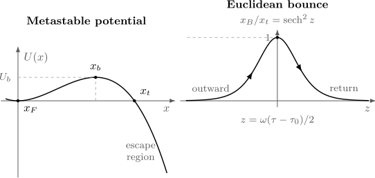
The false minimum $x_F$ is separated from the escape region by a barrier. In Euclidean time the bounce approaches $x_F$ at both ends, reaches $x_t$ at its center $\tau_0$, and returns. The cubic example below has an exact $\operatorname{sech}^2$ profile.

What the false vacuum means in zero spatial dimensions

In field theory, “vacuum” denotes a state associated with a homogeneous field configuration. In ordinary quantum mechanics, the corresponding object is a wavepacket or resonance localized near a metastable well. The terminology is useful, but the local minimum itself is not an exact stationary quantum state.

Two common realizations must be distinguished:

1. An open escape problem: the potential falls toward an unbounded or asymptotic region, and outgoing boundary conditions define a resonance with a complex energy.
2. A closed multiwell problem: the full Hamiltonian has a real discrete spectrum, but a state initially localized in one well can remain trapped for a long time before tunneling, dephasing, and eventually recurring.

A local minimum alone does not guarantee a useful exponential decay regime. The barrier must produce a parametrically long timescale, normally requiring a bounce action $B$ with

$$\frac{B}{\hbar}\gg1.$$

The Euclidean Boundary-Value Problem

Subtract the false-minimum background and define

$$B[x] = \int_{-\infty}^{\infty} d\tau \left[ \frac{m}{2}(x')^2 + U(x) \right].$$

Stationarity gives

$$mx'' = U'(x).$$

The bounce boundary conditions are

$$\begin{gathered} x_B(\tau)\to x_F, \qquad x_B'(\tau)\to0, \\ \tau\to\pm\infty, \\ x_B(\tau_0)=x_t, \qquad x_B'(\tau_0)=0. \end{gathered}$$

The solution is symmetric about its center:

$$x_B(\tau_0+\sigma) = x_B(\tau_0-\sigma).$$

Translation invariance makes $\tau_0$ arbitrary. This continuous family of equal-action solutions is the origin of the translation zero mode.

Inverted-potential interpretation

The Euclidean equation can be written

$$mx_B'' = - \frac{d}{dx_B} \left[ -U(x_B) \right].$$

In the mechanical analogy, a particle starts asymptotically at the unstable equilibrium on top of $-U$ at $x_F$, rolls to $x_t$, stops there, and retraces its path. It takes infinite Euclidean time to leave or return to the top because $x_F$ is approached exponentially.

The analogy constructs a stationary path. It does not describe the real-time motion of the quantum particle during tunneling.

First integral

Because the Euclidean Lagrangian has no explicit $\tau$ dependence,

$$\mathcal E_E = \frac{m}{2}(x_B')^2 - U(x_B)$$

is conserved. The asymptotic boundary conditions set $\mathcal E_E=0$, so

$$\frac{m}{2}(x_B')^2 = U(x_B).$$

On either half of the bounce,

$$\left| \frac{dx_B}{d\tau} \right| = \sqrt{ \frac{2U(x_B)}{m} }.$$

The implicit profile is therefore

$$\left| \tau-\tau_0 \right| = \sqrt{\frac{m}{2}} \int_{x_B(\tau)}^{x_t} \frac{dy}{\sqrt{U(y)}}.$$

Near $x_F$,

$$U(x) = \frac{m\omega_F^2}{2} (x-x_F)^2 + O\left( (x-x_F)^3 \right),$$

so the integral diverges logarithmically and

$$x_B(\tau)-x_F \propto e^{-\omega_F|\tau-\tau_0|}.$$

The Round-Trip Action

The zero-energy first integral reduces the action:

$$\begin{aligned} B &= \int_{-\infty}^{\infty} d\tau \left[ \frac{m}{2}(x_B')^2 + U(x_B) \right] \\ &= \int_{-\infty}^{\infty} d\tau\, 2U(x_B). \end{aligned}$$

The outward and return branches contribute equally. Hence

$$B = 2 \int_{x_F}^{x_t} dx\, \sqrt{2mU(x)}.$$

The factor of two is structural. A monotone instanton crosses once between degenerate minima; a bounce leaves and returns to the same minimum.

Relation to WKB

For a one-dimensional barrier, define the fixed-energy WKB action

$$W(E) = \int_{x_1(E)}^{x_2(E)} dx\, \sqrt{2m[U(x)-E]}.$$

At the classical false-minimum energy $E=0$,

$$B = 2W(0).$$

Therefore the bounce factor

$$e^{-B/\hbar}$$

matches the leading WKB probability suppression $e^{-2W/\hbar}$. A WKB wavefunction amplitude contains only $e^{-W/\hbar}$.

The false-well ground energy is actually of order $\hbar\omega_F/2$, not exactly zero. Using $W(E_F)$ shifts some subleading terms between exponent and prefactor. Agreement claims must state the approximation order and energy convention.

Worked Example: Cubic Metastable Potential

Consider

$$U(x) = \frac{m\omega^2}{2}x^2 - \frac{g}{3}x^3, \qquad g\gt0.$$

The false minimum is at $x_F=0$. The barrier top satisfies

$$x_b = \frac{m\omega^2}{g},$$

with height

$$U_b = \frac{m^3\omega^6}{6g^2}.$$

The nonzero root of $U(x)=0$ is

$$x_t = \frac{3m\omega^2}{2g}.$$

Exact bounce profile

The zero-energy equation is

$$(x_B')^2 = \omega^2x_B^2 \left( 1-\frac{x_B}{x_t} \right).$$

The solution centered at $\tau_0$ is

$$x_B(\tau) = x_t \operatorname{sech}^2 \left[ \frac{\omega}{2} (\tau-\tau_0) \right].$$

Indeed,

$$\begin{aligned} x_B' &= - \omega x_B \tanh \left[ \frac{\omega}{2} (\tau-\tau_0) \right], \\ 1-\frac{x_B}{x_t} &= \tanh^2 \left[ \frac{\omega}{2} (\tau-\tau_0) \right], \end{aligned}$$

so the first integral is satisfied on both branches.

Exact bounce action

Using the round-trip formula,

$$\begin{aligned} B &= 2m\omega \int_0^{x_t} dx\, x \sqrt{ 1-\frac{x}{x_t} } \\ &= \frac{8}{15} m\omega x_t^2 \\ &= \frac{6m^3\omega^5}{5g^2}. \end{aligned}$$

In terms of the barrier height,

$$B = \frac{36}{5} \frac{U_b}{\omega}.$$

The natural dimensionless coupling is

$$\lambda \equiv \frac{\hbar g^2} {m^3\omega^5},$$

for which

$$\frac{B}{\hbar} = \frac{6}{5\lambda}.$$

The bounce expansion is controlled when $\lambda\ll1$.

Zero and Negative Fluctuation Modes

Write

$$x(\tau) = x_B(\tau) + \eta(\tau).$$

The quadratic fluctuation operator is

$$\mathcal M_B = - m\frac{d^2}{d\tau^2} + U''(x_B).$$

Translation zero mode

Differentiate the bounce equation with respect to $\tau$:

$$m x_B''' = U''(x_B)x_B'.$$

Therefore

$$\mathcal M_B x_B' = 0.$$

The zero mode shifts the center $\tau_0$. It must be removed from the ordinary determinant and replaced by an integral over $\tau_0$.

Why one negative mode appears

The zero mode $x_B'$ changes sign once, at the center of the bounce. For a one-dimensional Sturm–Liouville operator on the Euclidean line, eigenfunctions are ordered by their number of nodes. A normalizable zero eigenfunction with one node has one lower eigenfunction with no nodes. Its eigenvalue is negative.

Thus a simple one-dimensional bounce has exactly one negative mode. This statement assumes the usual isolated bounce and self-adjoint fluctuation problem. Additional negative modes can signal a different saddle, an excited or oscillating solution, or an incorrectly chosen decay configuration.

Spectrum for the cubic bounce

For the cubic example,

$$\begin{aligned} \frac{\mathcal M_B}{m} &= - \frac{d^2}{d\tau^2} + \omega^2 \\ &\quad\times \left[ 1 - 3\operatorname{sech}^2 \left( \frac{\omega}{2} (\tau-\tau_0) \right) \right]. \end{aligned}$$

With

$$z = \frac{\omega}{2} (\tau-\tau_0),$$

this becomes the Pöschl–Teller operator

$$\mathcal M_B = \frac{m\omega^2}{4} \left[ - \frac{d^2}{dz^2} + 4 - 12\operatorname{sech}^2z \right].$$

Its negative and zero modes can be displayed explicitly:

$$\begin{array}{c|c} \text{mode} & \text{eigenvalue} \\ \hline \eta_-(z)\propto\operatorname{sech}^3z & -5m\omega^2/4 \\ \eta_0(z)\propto \operatorname{sech}^2z\,\tanh z & 0 \end{array}$$

The zero mode is proportional to $x_B'$. The remaining discrete positive mode and continuum affect the determinant prefactor but not the classical exponent.

From a Bounce to a Decay Exponent

For a long Euclidean interval of duration $T$, the arbitrary center produces a factor proportional to $T$. Widely separated bounces can then be summed in a dilute approximation. The negative mode specifies how the integration contour passes through the saddle and produces an imaginary contribution to the analytically continued false-well energy.

The resulting semiclassical structure is

$$E_{\mathrm{res}} = \mathcal E_F - \frac{i\hbar\Gamma}{2},$$

with

$$\Gamma \sim A e^{-B/\hbar} \left[ 1 + O\left( \frac{\hbar}{B} \right) \right].$$

The exponent is fixed by the classical bounce. The prefactor $A$ must have units of inverse time and depends on fluctuation determinants, zero-mode normalization, the negative-mode contour, and the definition of the metastable state.

This formula does not assert exact exponential decay at all times. Unitary quantum mechanics gives nonexponential behavior at sufficiently short and long times. The bounce result describes the resonance-dominated regime in which a decay rate is a useful emergent quantity.

Diluteness and repeated events

A one-bounce calculation is parametrically credible when:

$$\frac{B}{\hbar}\gg1, \qquad \frac{\Gamma}{\omega_F}\ll1.$$

The first condition suppresses each event; the second separates the bounce width, of order $1/\omega_F$, from the mean time between events. If bounces overlap strongly, their interactions and quasi-zero modes invalidate a naive Poisson sum.

Prefactor Caveats

The symbolic form $A e^{-B/\hbar}$ hides several logically distinct operations.

Ingredient	Why it matters
Reference determinant	Normalizes fluctuations relative to the false-well saddle
Translation zero mode	Replaces a vanishing determinant eigenvalue by an integral over $\tau_0$
One negative mode	Selects a contour and produces the imaginary part associated with decay
Boundary conditions	Distinguish a resonance, fixed-endpoint kernel, thermal trace, and closed system
State normalization	Fixes whether the answer is a kernel coefficient, energy width, or rate
Multi-bounce sum	Converts the one-event contribution into long-time extensive behavior

The familiar schematic zero-mode replacement,

$$\begin{aligned} (\det\mathcal M_B)^{-1/2} &\longrightarrow J_0 \int d\tau_0 \\ &\quad\times (\det{}'\mathcal M_B)^{-1/2}. \end{aligned}$$

contains a Jacobian $J_0$ whose precise form depends on the path-integral measure and normalization convention. The negative Gaussian direction is not convergent on the original real fluctuation contour; its continuation supplies an imaginary factor and a prescription-dependent half factor.

These details cannot be reconstructed from $B$ alone. Fluctuation Determinants Preview is the canonical home for the determinant ratio and collective-coordinate framework.

Numerical Construction

For a general one-dimensional potential, the first integral is usually more stable than direct shooting.

Quadrature route

1. Find $x_F$, the barrier top, and the first root $x_t$ beyond the barrier with $U(x_t)=U(x_F)$.
2. Shift $U(x_F)$ to zero.
3. Evaluate

$$B = 2 \int_{x_F}^{x_t} dx\, \sqrt{2mU(x)}.$$

4. Reconstruct the profile from

$$\left| \tau-\tau_0 \right| = \sqrt{\frac{m}{2}} \int_{x_B(\tau)}^{x_t} \frac{dy}{\sqrt{U(y)}}.$$

The integrable square-root behavior at $x_t$ and logarithmic divergence at $x_F$ should be handled with endpoint-aware quadrature or a change of variables.

Boundary-value route

On a finite symmetric interval $[-L,L]$, impose

$$x_B'(0)=0, \qquad x_B(L)\approx x_F,$$

and solve only on $[0,L]$. The center value approaches $x_t$ as $L\to\infty$. A boundary-value solver is usually more stable than launching exactly from $x_t$ with zero velocity, because the latter is sensitive to roundoff.

Diagnostics

A converged solution should satisfy:

• $\mathcal E_E=m(x_B')^2/2-U(x_B)\approx0$ along the path;
• direct $\tau$ integration and configuration-space quadrature agree for $B$;
• the endpoint error falls as $e^{-\omega_F L}$;
• the smallest odd fluctuation eigenvalue approaches zero as the grid is refined;
• exactly one lower eigenvalue remains negative;
• $B$ is stable under independent changes of $L$, mesh density, and quadrature rule.

The translation mode is an especially sensitive end-to-end check because it tests the profile, derivatives, fluctuation operator, and boundary truncation at once.

Competing and Generalized Bounces

Several real bounces can exist when a potential has multiple escape directions or intermediate wells. At leading exponential order, the smallest admissible action dominates:

$$B_{\mathrm{dom}} = \min_\alpha B_\alpha,$$

provided no symmetry, contour, or boundary condition excludes that saddle. Nearly equal actions require prefactors and interference information.

Other possibilities include:

• periodic bounces at finite temperature;
• energy-dependent periodic instantons;
• multidimensional bounces with more than one path through configuration space;
• complex saddles when no relevant real Euclidean solution exists;
• oscillating solutions with extra negative modes.

Not every stationary Euclidean solution controls a decay rate. Boundary data, contour accessibility, and fluctuation signature remain part of the selection rule.

Bridge to Field-Theory False Vacuum Decay

For one scalar field in $d$ spatial dimensions,

$$\begin{aligned} S_E[\phi] &= \int d\tau\,d^d x \\ &\quad\times \left[ \frac12(\partial_\tau\phi)^2 + \frac12(\boldsymbol\nabla\phi)^2 \right. \\ &\qquad\left. + V(\phi) \right]. \end{aligned}$$

Under the standard assumptions for a single scalar, the least-action bounce can be taken to be rotationally symmetric in $D=d+1$ Euclidean dimensions. With

$$\rho = \sqrt{ \tau^2+|\mathbf x|^2 },$$

the radial equation is

$$\frac{d^2\phi_B}{d\rho^2} + \frac{d}{\rho} \frac{d\phi_B}{d\rho} = V'(\phi_B),$$

with

$$\begin{gathered} \phi_B'(0)=0, \\ \phi_B(\rho)\to\phi_F \quad \text{as} \quad \rho\to\infty. \end{gathered}$$

The term $d\phi_B'/\rho$ acts like friction in the inverted-potential analogy. The mechanical energy obeys

$$\frac{d}{d\rho} \left[ \frac12(\phi_B')^2 - V(\phi_B) \right] = - \frac{d}{\rho} (\phi_B')^2 \leq0.$$

Quantum mechanics is the case $d=0$, where the friction term vanishes and the exact first integral is recovered. In field theory the center value is not generally the equal-potential turning point; it must be tuned so that friction leaves the solution at $\phi_F$ as $\rho\to\infty$. This is the basis of the overshoot–undershoot construction.

The field-theory exponent is

$$B = S_E[\phi_B] - S_E[\phi_F].$$

Gauge fields, fermions, renormalization, multiple scalar fields, gravity, and finite temperature add substantial structure. Bridge to QFT Instantons maps the saddle dictionary, while From Euclidean Time to Euclidean QFT owns the broader Euclidean-field and reconstruction framework.

Reliability Checklist

Before trusting a bounce exponent, verify:

1. Reference configuration: Is the false-minimum action subtracted?
2. Escape geometry: Does a turning point with the correct equal-potential value exist?
3. Boundary data: Does the path return to the same metastable configuration?
4. Finite action: Are the Euclidean tails normalizable and exponentially decaying?
5. Round trip: Has the factor of two in the one-dimensional action been included?
6. Semiclassical control: Is $B/\hbar\gg1$?
7. Mode count: Is there one translation zero mode and exactly one negative mode?
8. Prefactor units: Does the completed result have units of a decay rate?
9. Competing saddles: Are lower-action exits, complex saddles, or thermal saddles absent?
10. Independent check: Does WKB or direct resonance numerics reproduce the exponent?

Common Mistakes

• Calling any finite-action Euclidean solution a bounce without checking its endpoints.
• Confusing an instanton between degenerate minima with a bounce that returns to one false minimum.
• Omitting the return branch and losing a factor of two in $B$.
• Using the barrier top $x_b$ as the turning point; the bounce turns at $U(x_t)=U(x_F)$.
• Leaving the false-vacuum background in an infinite action.
• Treating the inverted-potential path as a real-time tunneling trajectory.
• Assuming the bounce is a minimum of $S_E$ even though it has one negative mode.
• Including the translation zero eigenvalue in an ordinary determinant.
• Quoting $e^{-B/\hbar}$ as a normalized rate without a prefactor and state convention.
• Assuming exponential decay is exact at arbitrarily short or long times.
• Copying the frictionless quantum-mechanical first integral into field theory.
• Choosing the lowest numerical action without checking contour accessibility and boundary conditions.

Exercises

1. Derive the bounce quadrature

Starting from

$$mx'' = U'(x),$$

derive the zero-energy first integral, the implicit bounce profile, and the round-trip action.

Solution

Multiply the equation by $x'$:

$$\frac{d}{d\tau} \left[ \frac{m}{2}(x')^2 - U(x) \right] = 0.$$

At $\tau\to\pm\infty$, both $x'$ and $U(x)$ vanish, so

$$\frac{m}{2}(x')^2 = U(x).$$

Separating variables on either branch gives

$$\left| \tau-\tau_0 \right| = \sqrt{\frac{m}{2}} \int_{x(\tau)}^{x_t} \frac{dy}{\sqrt{U(y)}}.$$

On shell, the kinetic and potential terms are equal. The two branches give

$$\begin{aligned} B &= 2 \int_{x_F}^{x_t} \frac{dx}{|x'|} \,2U(x) \\ &= 2 \int_{x_F}^{x_t} dx\, \sqrt{2mU(x)}. \end{aligned}$$

2. Explain the WKB factor of two

Let

$$W(0) = \int_{x_F}^{x_t} dx\, \sqrt{2mU(x)}.$$

Explain why the bounce exponent is $B=2W(0)$ and why this matches a tunneling probability rather than a wavefunction amplitude.

Solution

The bounce traverses the forbidden interval twice: once from $x_F$ to $x_t$ and once on the return branch. Each branch contributes $W(0)$, so

$$B = 2W(0).$$

In WKB, crossing the barrier suppresses a wavefunction amplitude by $e^{-W/\hbar}$. Squaring an amplitude produces a probability suppression

$$\left| e^{-W/\hbar} \right|^2 = e^{-2W/\hbar} = e^{-B/\hbar}.$$

Prefactors and the false-well oscillation scale are still needed to turn this probability per attempt into a rate.

3. Verify the cubic bounce and action

For

$$U(x) = \frac{m\omega^2}{2}x^2 - \frac{g}{3}x^3,$$

find $x_b$, $U_b$, and $x_t$. Verify the $\operatorname{sech}^2$ bounce and compute $B$.

Solution

The stationary points obey

$$U'(x) = x(m\omega^2-gx) = 0,$$

so the barrier top is

$$x_b = \frac{m\omega^2}{g}, \qquad U_b = \frac{m^3\omega^6}{6g^2}.$$

The nonzero root of $U(x)=0$ is

$$x_t = \frac{3m\omega^2}{2g}.$$

For

$$x_B = x_t\operatorname{sech}^2z, \qquad z = \frac{\omega}{2} (\tau-\tau_0),$$

one has

$$x_B' = -\omega x_B\tanh z$$

and

$$1-\frac{x_B}{x_t} = \tanh^2z.$$

Hence

$$(x_B')^2 = \omega^2x_B^2 \left( 1-\frac{x_B}{x_t} \right),$$

which is the first integral. Finally,

$$\begin{aligned} B &= 2m\omega x_t^2 \int_0^1 dy\, y(1-y)^{1/2} \\ &= 2m\omega x_t^2 \left( \frac{4}{15} \right) \\ &= \frac{6m^3\omega^5}{5g^2}. \end{aligned}$$

4. Count the negative modes

Show that $x_B'$ is a zero mode of $\mathcal M_B$. Use its node count to argue that a simple one-dimensional bounce has one negative mode.

Solution

Differentiating

$$mx_B'' = U'(x_B)$$

gives

$$mx_B''' = U''(x_B)x_B'.$$

Therefore

$$\left[ - m\frac{d^2}{d\tau^2} + U''(x_B) \right] x_B' = 0.$$

The bounce rises before $\tau_0$ and falls after it, so $x_B'$ changes sign once. The Sturm–Liouville node theorem orders normalizable eigenfunctions by node number. A zero mode with one node is the first excited fluctuation state; one nodeless eigenfunction lies below it and has negative eigenvalue. No second negative eigenvalue can lie below without violating the node ordering.

5. Estimate finite-interval errors

Suppose the tail is

$$x_B(\tau)-x_F \simeq C e^{-\omega_F|\tau|}.$$

Estimate the action omitted by truncating the Euclidean line to $[-L,L]$.

Solution

In the quadratic tail,

$$U \simeq \frac{m\omega_F^2}{2} (x_B-x_F)^2,$$

and the zero-energy relation makes the kinetic term equal to $U$. On the positive tail,

$$\begin{aligned} \delta B_+ &\simeq \int_L^\infty d\tau\, m\omega_F^2C^2 e^{-2\omega_F\tau} \\ &= \frac{m\omega_F C^2}{2} e^{-2\omega_F L}. \end{aligned}$$

The negative tail contributes equally, so

$$\delta B \simeq m\omega_F C^2 e^{-2\omega_F L}.$$

The endpoint displacement is of order $e^{-\omega_F L}$, while the action error is of order $e^{-2\omega_F L}$.

6. Derive Euclidean friction in field theory

For a radial field-theory bounce satisfying

$$\phi_B'' + \frac{d}{\rho}\phi_B' = V'(\phi_B),$$

show that the inverted-potential mechanical energy decreases with $\rho$. Explain why the quantum-mechanical equal-potential turning-point rule no longer holds for $d\gt0$.

Solution

Define

$$\mathcal E(\rho) = \frac12(\phi_B')^2 - V(\phi_B).$$

Then

$$\begin{aligned} \frac{d\mathcal E}{d\rho} &= \phi_B' \left[ \phi_B''-V'(\phi_B) \right] \\ &= - \frac{d}{\rho} (\phi_B')^2 \leq0. \end{aligned}$$

For $d=0$, the right-hand side vanishes and energy is conserved, so the center and false-vacuum endpoints lie at equal potential values. For $d\gt0$, friction removes mechanical energy as the trajectory moves outward in $\rho$. The center value must start farther up the inverted potential so that the damped trajectory approaches $\phi_F$ at infinity.

Cross-Links

• Instantons, Tunneling, and Nonperturbative Effects
• Euclidean Time and Imaginary-Time Action
• Instantons in Quantum Mechanics
• False Vacuum Decay in Quantum Mechanics
• Fluctuation Determinants Preview
• Double-Well Tunneling
• Barrier Penetration and Tunneling
• Instantons in Quantum Mechanics Preview
• Small Parameters and Error Estimates
• Bridge to QFT Instantons
• From Euclidean Time to Euclidean QFT

References

1. S. Coleman, “The Uses of Instantons”, in Aspects of Symmetry, Cambridge University Press, 1985, pp. 265–350. Canonical pedagogical account of bounces, dilute gases, and metastable decay.
2. S. Coleman, “Fate of the False Vacuum: Semiclassical Theory”, Physical Review D 15, 2929–2936 (1977), with erratum in 16, 1248 (1977). Foundational field-theory bounce construction and overshoot–undershoot argument.
3. C. G. Callan Jr. and S. Coleman, “Fate of the False Vacuum. II. First Quantum Corrections”, Physical Review D 16, 1762–1768 (1977). Fluctuation prefactor, zero mode, and decay-rate framework.
4. S. Coleman, V. Glaser, and A. Martin, “Action Minima among Solutions to a Class of Euclidean Scalar Field Equations,” Communications in Mathematical Physics 58, 211–221 (1978). Symmetry and least-action properties of scalar Euclidean bounces.
5. R. Rajaraman, Solitons and Instantons, North-Holland, 1982. Detailed finite-action solutions and fluctuation spectra.
6. J. Zinn-Justin, Path Integrals in Quantum Mechanics, Oxford University Press, 2005. Euclidean quantum mechanics, metastable potentials, and saddle expansions.
7. H. Kleinert, Path Integrals in Quantum Mechanics, Statistics, Polymer Physics, and Financial Markets, 5th ed., World Scientific, 2009. Broad treatment of bounce methods and functional determinants.
8. J. S. Langer, “Statistical Theory of the Decay of Metastable States”, Annals of Physics 54, 258–275 (1969). Foundational analytic-continuation and metastability framework.
9. I. Affleck, “Quantum-Statistical Metastability”, Physical Review Letters 46, 388–391 (1981). Quantum and thermal crossover in metastable decay.
10. G. Álvarez, “Coupling-Constant Behavior of the Resonances of the Cubic Anharmonic Oscillator”, Physical Review A 37, 4079–4083 (1988). Asymptotic and numerical resonance results for the cubic metastable oscillator.
11. A. Andreassen, D. Farhi, W. Frost, and M. D. Schwartz, “Direct Approach to Quantum Tunneling”, Physical Review Letters 117, 231601 (2016). Modern treatment clarifying tunneling-rate definitions and Euclidean methods.