False Vacuum Decay in Quantum Mechanics

A false vacuum in quantum mechanics is a long-lived state localized near a local minimum that can escape through a barrier. The word “vacuum” is inherited from field theory. In ordinary one-particle quantum mechanics, the relevant object is not the minimum of the potential itself and not an exact normalizable energy eigenstate. It is a metastable wavepacket, a quasibound level, or an outgoing resonance.

The central observable is a decay rate. With the convention

$$\mathcal E_F = E_R - \frac{i\hbar\gamma}{2},$$

the resonance-dominated survival probability behaves as

$$P_F(t) \simeq e^{-\gamma t}, \qquad \tau_F = \frac{1}{\gamma}.$$

Here $\gamma$ has units of inverse time, $\tau_F$ is the lifetime, and $\Gamma_E=\hbar\gamma$ is the corresponding energy width.

This page owns the observable interpretation of quantum-mechanical false-vacuum decay: state preparation, survival and nonescape probabilities, resonance poles, WKB escape rates, the range of validity of exponential decay, and the dictionary to field theory. Bounce Solutions owns the Euclidean boundary-value problem, bounce action, exact cubic example, and fluctuation-mode diagnostic. Fluctuation Determinants Preview owns determinant normalization and collective-coordinate prefactors.

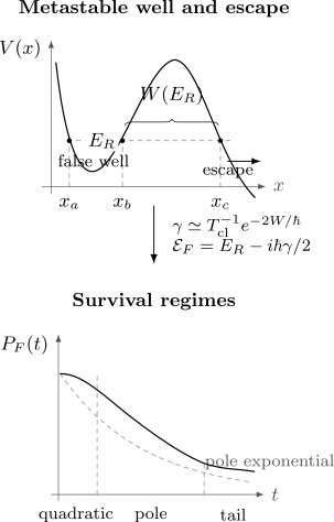
A quasibound level leaks through the forbidden interval between $x_b$ and $x_c$. The resulting exponential law is an intermediate-time approximation: unitary evolution begins quadratically and, for a Hamiltonian bounded below, ultimately develops a nonexponential threshold tail.

The Metastable Well

Let $V(x)$ have a local minimum at $x_F$:

$$V'(x_F)=0, \qquad V''(x_F)\gt0.$$

A barrier separates this false minimum from an escape region. Near $x_F$,

$$V(x) \simeq V_F + \frac{m\omega_F^2}{2} (x-x_F)^2,$$

so the well supports local oscillator-like levels. For the lowest one,

$$E_F \simeq V_F + \frac{\hbar\omega_F}{2},$$

before tunneling and anharmonic corrections are included.

The local level is not generally an eigenvalue of the full self-adjoint Hamiltonian. If the potential opens into a continuum, probability can escape and an outgoing resonance replaces the putative bound state. If the entire potential is confining, the exact spectrum remains real and discrete; leakage from one well is then followed by interference and recurrence rather than irreversible decay.

This distinction is foundational:

• Open escape geometry: outgoing boundary conditions define a resonance and an approximate decay rate.
• Closed finite geometry: exact evolution is quasiperiodic; a rate can describe only a coarse-grained or intermediate-time loss from a chosen region.
• Open-system geometry: environmental degrees of freedom may make exponential relaxation accurate over a wider interval, but the rate then depends on the system–environment model.

Calling a local minimum a false vacuum therefore abbreviates a state-preparation and boundary-condition problem.

Preparing the false-well state

One practical preparation is a normalized packet $\lvert F\rangle$ concentrated inside the well. Another is to confine the system temporarily, prepare a local eigenstate, and then remove the auxiliary wall. Either construction introduces details that affect early transients but not the leading semiclassical exponent when the barrier is high.

Choose a dividing point $x_d$ beyond the barrier and define a false-well projector, schematically,

$$\Pi_F = \Theta(x_d-\hat x).$$

The nonescape probability is

$$P_{\mathrm{ne}}(t) = \langle\psi(t)\vert \Pi_F \vert\psi(t)\rangle.$$

The survival probability of the initially prepared state is

$$P_{\mathrm{surv}}(t) = \left| \langle F\vert e^{-iHt/\hbar} \vert F\rangle \right|^2.$$

These observables are not identical. A packet can deform or dephase within the well, reducing its overlap with $\lvert F\rangle$ without having escaped. For an isolated narrow resonance after preparation transients have died away, both quantities often exhibit the same dominant exponential rate.

Flux, Survival, and Resonance

The three most useful descriptions emphasize different data:

Description	Defining quantity	What it measures
Nonescape	$\langle\Pi_F\rangle_t$	Probability remaining in a chosen well region
Survival	$\lvert\langle F\vert e^{-iHt/\hbar}\vert F\rangle\rvert^2$	Persistence of the specific prepared state
Resonance	Pole $\mathcal E_F=E_R-i\hbar\gamma/2$	Energy, width, and intermediate-time decay scale

For one escape boundary, the continuity equation gives

$$\frac{dP_{\mathrm{ne}}}{dt} = - j(x_d,t),$$

where

$$j(x,t) = \frac{\hbar}{m} \operatorname{Im} \left[ \psi^*(x,t) \frac{\partial\psi(x,t)}{\partial x} \right].$$

An instantaneous loss rate can be defined whenever $P_{\mathrm{ne}}(t)\gt0$:

$$\gamma_{\mathrm{inst}}(t) = - \frac{d}{dt} \ln P_{\mathrm{ne}}(t) = \frac{j(x_d,t)}{P_{\mathrm{ne}}(t)}.$$

It is approximately constant only in the exponential window. This flux definition makes clear that a decay rate is an observable statement about probability leaving a region, not merely the exponential of a Euclidean action.

Outgoing resonances

A one-dimensional resonance solves the stationary Schrödinger equation with an outgoing-wave condition in the escape channel. Schematically,

$$\psi_{\mathrm{res}}(x) \sim e^{+ikx} \qquad (x\to+\infty),$$

with no incoming component. The resulting complex energy

$$\mathcal E_F = E_R - \frac{i\Gamma_E}{2}$$

is a pole of the analytically continued resolvent or scattering matrix, usually on a nonphysical sheet. Its formal time dependence is

$$e^{-i\mathcal E_F t/\hbar} = e^{-iE_Rt/\hbar} e^{-\Gamma_Et/(2\hbar)}.$$

Taking the modulus squared gives

$$P_F(t) \propto e^{-\Gamma_Et/\hbar} = e^{-\gamma t}, \qquad \gamma = \frac{\Gamma_E}{\hbar}.$$

The outgoing resonance function is generally not square-integrable. It is a compact representation of the pole contribution to physical wavepacket evolution, not an ordinary Hilbert-space eigenvector.

Why Decay Is Only Approximately Exponential

Define the survival amplitude

$$\mathcal A_F(t) = \langle F\vert e^{-iHt/\hbar} \vert F\rangle.$$

By the spectral theorem,

$$\mathcal A_F(t) = \int_{E_{\min}}^\infty \rho_F(E) e^{-iEt/\hbar} \,dE,$$

where

$$\rho_F(E) = \langle F\vert \delta(E-H) \vert F\rangle.$$

Normalization requires

$$\int_{E_{\min}}^\infty \rho_F(E)\,dE = 1.$$

A narrow resonance produces an approximately Breit–Wigner peak,

$$\begin{aligned} \rho_F(E) &\simeq \rho_{\mathrm{pole}}(E) + \rho_{\mathrm{bg}}(E), \\ \rho_{\mathrm{pole}}(E) &= \frac{Z\Gamma_E}{2\pi D(E)}, \\ D(E) &= (E-E_R)^2 + (\Gamma_E/2)^2. \end{aligned}$$

Fourier transforming the isolated pole contribution gives the exponential law. The background, the physical threshold $E_{\min}$, and the details of state preparation generate deviations.

Short times: the quadratic law

Assuming the required energy moments through fourth order are finite, expanding the unitary evolution gives

$$\begin{aligned} \mathcal A_F(t) &= 1 - \frac{i\langle H\rangle_F}{\hbar}t \\ &\quad- \frac{\langle H^2\rangle_F}{2\hbar^2}t^2 O(t^3). \end{aligned}$$

Consequently,

$$P_{\mathrm{surv}}(t) = 1 - \frac{(\Delta H)_F^2}{\hbar^2}t^2 + O(t^4).$$

Thus the initial slope vanishes:

$$\left. \frac{dP_{\mathrm{surv}}}{dt} \right|_{t=0} = 0.$$

The scale

$$\tau_Z = \frac{\hbar}{(\Delta H)_F}$$

is often called the Zeno time. An exact exponential would have a nonzero negative slope at $t=0$, so it cannot describe sufficiently short unitary evolution of a state with finite energy variance.

Intermediate times: pole dominance

After preparation transients and before threshold effects dominate, a narrow isolated pole can control the Fourier integral:

$$\mathcal A_F(t) \simeq Z_{\mathrm{pole}} e^{-iE_Rt/\hbar} e^{-\gamma t/2},$$

and therefore

$$P_{\mathrm{surv}}(t) \simeq \lvert Z_{\mathrm{pole}}\rvert^2 e^{-\gamma t}.$$

This is the regime computed by standard WKB and bounce methods. A useful lifetime requires

$$\gamma \ll \omega_F,$$

so intrawell motion and preparation transients occur on a much shorter timescale than escape.

Long times: the threshold tail

Because a physical Hamiltonian is bounded below, its spectral density cannot be an exact Lorentzian over the entire real axis. Suppose near threshold

$$\rho_F(E) \sim C(E-E_{\min})^\alpha, \qquad \alpha\gt-1.$$

Then the endpoint of the spectral integral gives

$$\begin{aligned} \mathcal A_F(t) &\sim C\, \Gamma(\alpha+1) e^{-iE_{\min}t/\hbar} \\ &\quad\times e^{-i\pi(\alpha+1)/2} \left( \frac{\hbar}{t} \right)^{\alpha+1}. \end{aligned}$$

so

$$P_{\mathrm{surv}}(t) \propto t^{-2(\alpha+1)}.$$

The crossover usually occurs only after many lifetimes because the pole contribution must first become extremely small. Nevertheless, the tail is conceptually essential: exact exponential decay for all $t\geq0$ is incompatible with a lower-bounded self-adjoint Hamiltonian.

WKB Escape Rate

Consider a quasibound level of energy $E$ with three turning points

$$x_a \lt x_b \lt x_c.$$

The interval $x_a\lt x\lt x_b$ is the classically allowed false well, while $x_b\lt x\lt x_c$ is the forbidden barrier. Define

$$p(x;E) = \sqrt{2m[E-V(x)]}$$

in the well and

$$\kappa(x;E) = \sqrt{2m[V(x)-E]}$$

under the barrier. The one-way forbidden action is

$$W(E) = \int_{x_b}^{x_c} \kappa(x;E)\,dx.$$

To leading exponential accuracy, the transmission probability per encounter with the barrier is

$$\mathcal T(E) \sim e^{-2W(E)/\hbar}.$$

The classical period of motion inside the false well is

$$T_{\mathrm{cl}}(E) = 2 \int_{x_a}^{x_b} \frac{m\,dx}{p(x;E)}.$$

For one escape barrier encountered once per period, the Gamow estimate is

$$\gamma_{\mathrm{WKB}}(E) \simeq \frac{1}{T_{\mathrm{cl}}(E)} e^{-2W(E)/\hbar}.$$

Near a harmonic false minimum,

$$T_{\mathrm{cl}} \simeq \frac{2\pi}{\omega_F},$$

and hence

$$\gamma_{\mathrm{WKB}} \simeq \frac{\omega_F}{2\pi} e^{-2W(E_F)/\hbar}.$$

The interpretation is “attempt frequency times escape probability per attempt.” It is reliable when the barrier transmission is small and successive encounters lose phase coherence into an effectively open escape channel.

What the simple prefactor omits

The factor $1/T_{\mathrm{cl}}$ is not a universal one-loop prefactor. Quantitative work may require:

• connection formulas at all turning points;
• the correct outgoing normalization and channel multiplicity;
• the energy shift of the quasibound level;
• barrier-top corrections when $W/\hbar$ is not large;
• interference from several escape paths;
• multidimensional stability determinants;
• environmental recrossing or dissipation.

The robust statement is

$$\ln\left( \frac{\gamma}{\omega_F} \right) = - \frac{2W}{\hbar} + O\!\left( \ln\frac{W}{\hbar} \right)$$

in a controlled high-barrier family. Prefactor accuracy requires more information than the leading exponent.

Bounce Estimate

The Euclidean bounce starts at the false minimum, reaches the far side of the barrier, and returns. For a one-dimensional fixed-energy problem, its background-subtracted action satisfies

$$\begin{aligned} B(E) &= 2 \int_{x_b}^{x_c} \sqrt{2m[V(x)-E]} \,dx \\ &= 2W(E). \end{aligned}$$

Thus

$$e^{-B(E)/\hbar} = e^{-2W(E)/\hbar},$$

matching the WKB probability suppression. The factor of two is geometric: the Euclidean bounce is a round trip, whereas $W$ is a one-way forbidden action.

At leading semiclassical order,

$$\gamma_{\mathrm{bounce}} \simeq A e^{-B/\hbar},$$

where $A$ has units of inverse time. The saddle action controls the exponential; the translation zero mode, the one negative mode, the determinant ratio, and normalization of the false-well state determine how the saddle contribution becomes a physical rate.

Equivalently, the metastable energy acquires

$$\operatorname{Im}\mathcal E_F = - \frac{\hbar\gamma}{2}.$$

In the standard Euclidean treatment, the negative fluctuation direction is handled by a contour prescription and supplies the imaginary contribution. It should not be discarded as a failed Gaussian integral. At the same time, an imaginary part does not arise from an ordinary finite-dimensional Hermitian eigenvalue problem without analytic continuation or outgoing boundary conditions. The physical observable and contour prescription are part of the calculation.

Bounce Solutions derives $B$, the boundary conditions, and the mode count. Fluctuation Determinants Preview explains why $A$ is a normalized determinant ratio rather than an arbitrary attempt frequency.

Three Routes to the Same Lifetime

Route	Primary input	Output	Strongest check
Real-time flux	Prepared packet and dividing surface	$P_{\mathrm{ne}}(t)$ and $\gamma_{\mathrm{inst}}(t)$	Plateau in the instantaneous rate
Resonance pole	Outgoing boundary condition	$E_R$ and $\Gamma_E=\hbar\gamma$	Stability under numerical exterior treatment
WKB or bounce	Barrier action and semiclassical fluctuations	Asymptotic exponent and prefactor	Agreement of $\ln\gamma$ across parameter scans

These methods need not agree pointwise outside their common regime. A time-dependent packet contains preparation transients and background continuum contributions. A resonance pole isolates one analytic structure. A bounce expansion is asymptotic in a semiclassical parameter. Agreement should be demanded after the same potential, energy convention, channel count, and normalization are imposed.

Numerical extraction

Several complementary calculations are useful:

1. Outgoing resonance: use complex scaling, an absorbing exterior, or a direct outgoing boundary condition to find $\mathcal E_F$.
2. Real-time propagation: initialize a packet in the false well and monitor $P_{\mathrm{ne}}(t)$ and the outgoing flux.
3. WKB quadrature: evaluate $W(E_R)$ and $T_{\mathrm{cl}}(E_R)$ using the same quasibound energy.
4. Euclidean saddle: solve the bounce problem and compare $B$ with $2W$.
5. Parameter scan: vary mass, barrier height, or a small coupling and compare the logarithmic slope of the exact and semiclassical rates.

A fitted exponential should be accompanied by a time window. Fitting across the initial quadratic region, a reflection from a numerical boundary, or the onset of a recurrence produces a number that is not a resonance lifetime.

From Quantum Mechanics to Field Theory

The quantum-mechanical problem is the zero-spatial-dimensional model of false-vacuum decay. The structural dictionary is:

Quantum mechanics	Scalar field theory
Coordinate $x(\tau)$	Field configuration $\phi(\tau,\mathbf x)$
False-well packet or resonance	State localized near a false-vacuum configuration
Barrier in $V(x)$	Barrier in the field configuration-space energy functional
Bounce $x_B(\tau)$	Euclidean bubble $\phi_B(\tau,\mathbf x)$
Rate $\gamma$	Decay rate per spatial volume $\Gamma/V$
One translation zero mode	Spacetime translation zero modes

For a scalar field in $3+1$ dimensions without gravity, the leading zero-temperature result has the form

$$\frac{\Gamma}{V} \simeq \mathcal A e^{-B/\hbar},$$

with

$$B = S_E[\phi_B] - S_E[\phi_F].$$

Under the assumptions of Euclidean invariance and a single scalar field, the least-action bounce is $O(4)$ symmetric. Writing

$$\rho = \sqrt{\tau^2+\mathbf x^2},$$

its radial equation is

$$\frac{d^2\phi}{d\rho^2} + \frac{3}{\rho} \frac{d\phi}{d\rho} = \frac{dV}{d\phi},$$

with

$$\left. \frac{d\phi}{d\rho} \right|_{\rho=0} = 0, \qquad \phi(\rho\to\infty) = \phi_F.$$

The extra term $3\phi'/\rho$ has no analogue in one-dimensional Euclidean quantum mechanics; it acts like radial friction in the inverted-potential picture. Four spacetime translation zero modes replace the single bounce-center zero mode, and the completed prefactor must have units of rate per volume.

The bridge has limits:

• finite-temperature decay is usually governed by an $O(3)$ thermal bounce rather than an $O(4)$ zero-temperature bounce;
• gauge fields and multiple scalar fields complicate the fluctuation problem;
• gravity changes both the saddle equations and the interpretation of decay;
• in finite volume, exact energy eigenstates remain real and the irreversible rate is again an asymptotic, large-volume, or coarse-grained concept.

Bridge to QFT Instantons places this dictionary beside other Euclidean saddles. The field-theory construction itself should be studied in its canonical QFT treatment rather than inferred by replacing $x$ with $\phi$ mechanically.

Reliability Checklist

Before quoting a false-vacuum lifetime, check:

1. State: What precisely is prepared near the false minimum?
2. Observable: Is the calculation about survival, nonescape, outgoing flux, a pole width, or a Euclidean persistence amplitude?
3. Boundary condition: Does the model have a genuine escape continuum or only a finite discrete spectrum?
4. Convention: Is the quoted $\Gamma$ an energy width or a rate?
5. Energy: Is the barrier action evaluated at $V_F$, at the local zero-point energy, or at a specified excited level?
6. Hierarchy: Are $\gamma\ll\omega_F$ and $W/\hbar\gg1$ satisfied?
7. Saddle: Does the bounce have the required endpoints and exactly one relevant negative mode?
8. Prefactor: Do the determinant, zero-mode, and channel factors give inverse-time units?
9. Window: Over what time interval is exponential decay actually observed?
10. Independent check: Do flux propagation, resonance numerics, WKB, and the bounce agree at least in the exponent?

Common Mistakes

• Treating the local minimum $x_F$ as a quantum state.
• Calling a normalizable eigenstate of a closed Hermitian Hamiltonian unstable.
• Writing $\mathcal E=E_R-i\gamma/2$ while also calling $\gamma$ a rate; the factor of $\hbar$ is then missing.
• Confusing survival probability with probability remaining inside the well.
• Using a one-way amplitude exponent $e^{-W/\hbar}$ as the decay probability.
• Evaluating $W$ at the bottom of the potential without stating whether zero-point energy is neglected.
• Treating the WKB attempt frequency as a universal determinant prefactor.
• Fitting a single exponential through the short-time quadratic regime or a late recurrence.
• Removing the bounce negative mode instead of specifying its contour treatment.
• Assuming the quantum-mechanical bounce equation transfers unchanged to field theory.

Exercises

1. Derive the short-time survival law

For a normalized state $\lvert F\rangle$ with finite energy moments through fourth order, expand the survival probability through order $t^2$ and show that its initial slope vanishes.

Solution

Expand the amplitude:

$$\begin{aligned} \mathcal A_F(t) &= 1 - \frac{i\langle H\rangle_F}{\hbar}t \\ &\quad- \frac{\langle H^2\rangle_F}{2\hbar^2}t^2 + O(t^3). \end{aligned}$$

Multiplying by its complex conjugate gives

$$P_{\mathrm{surv}}(t) = \lvert\mathcal A_F(t)\rvert^2.$$

Expanding the product,

$$\begin{aligned} P_{\mathrm{surv}}(t) &= 1 - \frac{\langle H^2\rangle_F}{\hbar^2} t^2 \\ &\quad+ \frac{\langle H\rangle_F^2}{\hbar^2} t^2 + O(t^4). \end{aligned}$$

Using the variance,

$$P_{\mathrm{surv}}(t) = 1 - \frac{(\Delta H)_F^2}{\hbar^2} t^2 + O(t^4).$$

Therefore

$$\dot P_{\mathrm{surv}}(0)=0.$$

The absence of a linear term is a consequence of unitary evolution, not of a tunneling approximation.

2. Convert a resonance energy into a lifetime

Suppose an outgoing resonance has

$$\mathcal E = E_R - \frac{i\Gamma_E}{2}.$$

Find its probability decay law, rate, and lifetime.

Solution

The pole contribution evolves as

$$e^{-i\mathcal E t/\hbar} = e^{-iE_Rt/\hbar} e^{-\Gamma_Et/(2\hbar)}.$$

Its modulus squared is

$$P(t) \propto e^{-\Gamma_Et/\hbar}.$$

Hence

$$\gamma = \frac{\Gamma_E}{\hbar}, \qquad \tau = \frac{1}{\gamma} = \frac{\hbar}{\Gamma_E}.$$

The distinction between $\Gamma_E$ and $\gamma$ prevents a common dimensional error.

3. Recover the attempt-frequency estimate

A packet in a nearly harmonic false well encounters one escape barrier once per classical period. The probability of transmission per encounter is $\mathcal T\ll1$. Derive the leading rate and specialize to frequency $\omega_F$.

Solution

After $N$ statistically independent encounters, the probability of remaining is

$$P_N = (1-\mathcal T)^N \simeq e^{-N\mathcal T}.$$

With $N\simeq t/T_{\mathrm{cl}}$,

$$P(t) \simeq \exp\left( - \frac{\mathcal T}{T_{\mathrm{cl}}}t \right).$$

Thus

$$\gamma \simeq \frac{\mathcal T}{T_{\mathrm{cl}}}.$$

For a harmonic well,

$$T_{\mathrm{cl}} = \frac{2\pi}{\omega_F},$$

and WKB gives

$$\gamma \simeq \frac{\omega_F}{2\pi} e^{-2W/\hbar}.$$

If there are two equivalent escape barriers encountered once each per period, the leading channel count doubles this result.

4. Derive a threshold power law

Assume

$$\rho_F(E) = C(E-E_{\min})^\alpha$$

near threshold, with $\alpha\gt-1$. Derive the leading long-time survival probability.

Solution

Set $\epsilon=E-E_{\min}$. The threshold contribution is

$$\mathcal A_F(t) \sim C e^{-iE_{\min}t/\hbar} \int_0^\infty \epsilon^\alpha e^{-i\epsilon t/\hbar} \,d\epsilon.$$

Rescale $u=\epsilon t/\hbar$:

$$\begin{aligned} \mathcal A_F(t) &\sim C e^{-iE_{\min}t/\hbar} \left( \frac{\hbar}{t} \right)^{\alpha+1} \\ &\quad\times \int_0^\infty u^\alpha e^{-iu}\,du. \end{aligned}$$

The regulated oscillatory integral is

$$\int_0^\infty u^\alpha e^{-iu}\,du = e^{-i\pi(\alpha+1)/2} \Gamma(\alpha+1).$$

Therefore

$$\begin{aligned} \mathcal A_F(t) &\propto t^{-(\alpha+1)}, \\ P_{\mathrm{surv}}(t) &\propto t^{-2(\alpha+1)}. \end{aligned}$$

5. Match the WKB and bounce exponents

For a fixed energy $E$, let

$$W(E) = \int_{x_b}^{x_c} \sqrt{2m[V(x)-E]} \,dx.$$

Explain why the bounce exponent is $B(E)=2W(E)$ and identify the corresponding WKB quantity.

Solution

The one-way forbidden WKB amplitude is suppressed by

$$e^{-W(E)/\hbar}.$$

A probability is quadratic in that amplitude:

$$\mathcal T(E) \sim e^{-2W(E)/\hbar}.$$

The Euclidean bounce travels from the false-well turning point to the far turning point and returns. Its background-subtracted geometric action therefore contains the forbidden integral twice:

$$B(E) = 2W(E).$$

Consequently,

$$e^{-B(E)/\hbar} = e^{-2W(E)/\hbar},$$

which matches the WKB transmission probability per escape attempt.

6. Explain why a closed two-level model does not decay

Let a normalized initial state have support on two exact eigenstates:

$$\lvert F\rangle = c_1\lvert E_1\rangle + c_2\lvert E_2\rangle.$$

Compute its survival probability and explain why no constant positive decay rate exists.

Solution

The survival amplitude is

$$\mathcal A_F(t) = \lvert c_1\rvert^2 e^{-iE_1t/\hbar} + \lvert c_2\rvert^2 e^{-iE_2t/\hbar}.$$

Therefore

$$\begin{aligned} P_{\mathrm{surv}}(t) &= \lvert c_1\rvert^4 + \lvert c_2\rvert^4 \\ &\quad+ 2 \lvert c_1c_2\rvert^2 \cos\left( \frac{E_2-E_1}{\hbar}t \right). \end{aligned}$$

The result oscillates and recurs. It cannot equal $e^{-\gamma t}$ with constant $\gamma\gt0$. Irreversible decay requires a continuum, an appropriate large-system limit, environmental coarse-graining, or an explicitly limited time window.

Cross-Links

• Instantons, Tunneling, and Nonperturbative Effects separates transmission, splitting, and decay observables.
• Bounce Solutions derives the bounce boundary conditions, action, and mode spectrum.
• Barrier Penetration and Tunneling owns the direct WKB transmission calculation.
• Euclidean Time and Imaginary-Time Action develops continuation, background subtraction, and fixed-energy exponents.
• Fluctuation Determinants Preview explains determinant ratios, zero modes, and negative modes.
• Small Parameters and Error Estimates gives the general language for asymptotic reliability.
• Bridge to QFT Instantons compares quantum-mechanical and field-theory Euclidean saddles.

References

1. G. Gamow, “Zur Quantentheorie des Atomkernes”, Zeitschrift für Physik 51, 204–212 (1928). Foundational barrier-penetration treatment of nuclear decay.
2. L. A. Khalfin, “Contribution to the Decay Theory of a Quasi-Stationary State”, Soviet Physics JETP 6, 1053–1063 (1958). Classic proof of nonexponential long-time behavior for lower-bounded spectra.
3. J. S. Langer, “Statistical Theory of the Decay of Metastable States”, Annals of Physics 54, 258–275 (1969). Foundational metastability, analytic-continuation, and rate framework.
4. L. Fonda, G. C. Ghirardi, and A. Rimini, “Decay Theory of Unstable Quantum Systems”, Reports on Progress in Physics 41, 587–631 (1978). Comprehensive account of survival amplitudes, resonances, and nonexponential regimes.
5. S. Coleman, “Fate of the False Vacuum: Semiclassical Theory”, Physical Review D 15, 2929–2936 (1977), with erratum in 16, 1248. Canonical field-theory bounce and false-vacuum construction.
6. C. G. Callan Jr. and S. Coleman, “Fate of the False Vacuum. II. First Quantum Corrections”, Physical Review D 16, 1762–1768 (1977). Fluctuation prefactor and decay-rate normalization.
7. S. Coleman, “The Uses of Instantons”, in Aspects of Symmetry, Cambridge University Press, 1985, pp. 265–350. Pedagogical quantum-mechanical bounce and dilute-gas treatment.
8. A. Andreassen, D. Farhi, W. Frost, and M. D. Schwartz, “Direct Approach to Quantum Tunneling”, Physical Review Letters 117, 231601 (2016). Physical decay-rate definition from real-time evolution and its relation to Euclidean methods.
9. A. Andreassen, D. Farhi, W. Frost, and M. D. Schwartz, “Precision Decay Rate Calculations in Quantum Field Theory”, Physical Review D 95, 085011 (2017). Careful normalization and higher-order structure of semiclassical decay rates.
10. G. Álvarez, “Coupling-Constant Behavior of the Resonances of the Cubic Anharmonic Oscillator”, Physical Review A 37, 4079–4083 (1988). Resonance asymptotics for a standard metastable quantum-mechanical model.
11. J. Zinn-Justin, Path Integrals in Quantum Mechanics, Oxford University Press, 2005. Systematic treatment of Euclidean saddles, metastable potentials, and semiclassical expansions.