Asymptotic Series and Nonperturbative Corrections

A perturbative calculation can be accurate even when its infinite series diverges. The apparent paradox disappears once two limits are kept separate. An asymptotic expansion controls the error as a parameter $g$ tends to zero at each fixed truncation order. Convergence would instead control the limit of the partial sums as the truncation order tends to infinity at fixed nonzero $g$.

In many quantum problems, perturbative coefficients eventually grow like $n!$. The terms first decrease, reach a least term near an order of size $1/g$, and then increase. The most accurate raw perturbative approximation is usually obtained by stopping near that least term. Its irreducible error is often exponentially small,

$$\text{least-term scale} \sim e^{-A/g},$$

which is also the characteristic size of tunneling and saddle contributions.

This page owns the physical meaning of that statement: factorial growth, optimal truncation, beyond-all-orders corrections, the invisibility of tunneling splittings to a local power series, and the quartic oscillator as the standard laboratory. Asymptotic Analysis owns the mathematical notation, Higher-Order Structure owns perturbative recursion, and Resurgence Preview owns Borel transforms, transseries, and ambiguity cancellation.

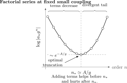
For coefficients of order $n!A^{-n}$, consecutive term magnitudes have ratio approximately $ng/A$. Terms decrease until $n$ reaches $n_*\simeq A/g$ and grow thereafter. The least term has the same exponential scale, $e^{-A/g}$, as effects that are invisible to every fixed power of $g$.

Convergent and Asymptotic Expansions

Suppose a quantity has a formal expansion

$$F(g) \sim \sum_{n=0}^{\infty} a_n g^n, \qquad g\to0^+.$$

The asymptotic symbol means that, for every fixed nonnegative integer $N$,

$$F(g) - \sum_{n=0}^{N} a_n g^n = o(g^N) \qquad \text{as }g\to0^+.$$

One often has the sharper estimate

$$F(g) - \sum_{n=0}^{N} a_n g^n = O(g^{N+1}),$$

but the constant hidden in the $O$ symbol may grow rapidly with $N$. Nothing in either statement requires

$$\lim_{N\to\infty} \sum_{n=0}^{N} a_n g^n$$

to exist at fixed $g\ne0$.

A convergent Taylor series and an asymptotic series therefore answer different questions.

Property	Convergent power series	Asymptotic power series
Limit being controlled	$N\to\infty$ at fixed $g$	$g\to0$ at fixed $N$
Effect of adding terms	Eventually improves the sum inside the convergence disk	Improves the approximation only while terms decrease
Remainder	Tends to zero as $N\to\infty$	Often smallest near a finite, $g$-dependent order
Uniqueness	Determines its sum in the convergence disk	Does not determine exponentially small additions by itself

The last row is the gateway to nonperturbative physics. Two functions that differ by $e^{-A/g}$ have the same power-series asymptotic expansion as $g\to0^+$. Local power-series data alone cannot decide which function a physical boundary-value problem selects.

An Exactly Solvable Model

Consider, for $g\gt0$,

$$I(g) = \int_0^\infty \frac{e^{-x}}{1+gx} \,dx.$$

This integral is finite and unambiguous. The finite geometric identity

$$\frac{1}{1+gx} = \sum_{n=0}^{N} (-gx)^n + \frac{(-gx)^{N+1}}{1+gx}$$

gives an exact decomposition after integration:

$$I(g) = \sum_{n=0}^{N} (-1)^n n!g^n + R_N(g),$$

where

$$R_N(g) = (-g)^{N+1} \int_0^\infty \frac{e^{-x}x^{N+1}}{1+gx} \,dx.$$

For each fixed $N$,

$$\lvert R_N(g)\rvert \lt (N+1)!g^{N+1},$$

so

$$I(g) \sim \sum_{n=0}^{\infty} (-1)^n n!g^n.$$

The expansion is asymptotic. It cannot converge for any nonzero $g$, because the ratio of consecutive term magnitudes is

$$\frac{(n+1)!g^{n+1}}{n!g^n} = (n+1)g,$$

which eventually exceeds one no matter how small $g$ is.

The exact answer can also be written

$$I(g) = \frac{e^{1/g}}{g} E_1\left(\frac{1}{g}\right),$$

where

$$E_1(z) = \int_z^\infty \frac{e^{-t}}{t} \,dt.$$

Thus a perfectly smooth, exactly defined function can possess a divergent weak-coupling expansion. Divergence is not evidence that the function or the original problem is ill-defined.

At $g=0.1$, the term magnitudes are

$$1,\; 0.1,\; 0.02,\; 0.006,\; 0.0024,\; \ldots$$

and reach their minimum near $n=9$ or $10$. The first several partial sums improve rapidly. Summing indefinitely would eventually destroy that accuracy.

What the model does and does not prove

Because the model series alternates and the exact remainder has a definite sign, its first omitted term supplies a useful bound. A general quantum perturbation series need not have either property. Its coefficients may have several competing large-order contributions, complex phases, logarithms, or singularities on different rays of the coupling plane.

The durable lesson is narrower:

1. factorial coefficient growth is compatible with an accurate low-order approximation;
2. the useful truncation order depends on the numerical value of the small parameter;
3. the smallest attainable raw perturbative error can be exponentially small.

Factorial Growth and Optimal Truncation

Assume the large-order coefficients behave as

$$a_n \sim C A^{-n} \Gamma(n+\beta), \qquad A\gt0.$$

The $n$th term is $T_n(g)=a_ng^n$. At large $n$,

$$\left| \frac{T_{n+1}(g)} {T_n(g)} \right| \sim \frac{g}{A} (n+\beta).$$

The terms stop decreasing when this ratio reaches one, so the optimal order is approximately

$$N_* \simeq \frac{A}{g} -\beta.$$

Since $N_*$ must be an integer, one compares the neighboring terms and truncates at the smaller one. The formula is an asymptotic estimate, not a command to retain a fractional number of terms.

To estimate the least term, set $z=N_*+\beta\simeq A/g$ and use Stirling’s formula:

$$\Gamma(z) \sim \sqrt{2\pi}\, z^{z-\frac12} e^{-z}.$$

Then

$$\begin{aligned} \lvert T_{N_*}(g)\rvert &\sim \lvert C\rvert A^{-N_*} \Gamma(N_*+\beta) g^{N_*} \\ &\sim \lvert C\rvert \sqrt{2\pi} \left( \frac{A}{g} \right)^{\beta-\frac12} e^{-A/g}. \end{aligned}$$

The power multiplying the exponential depends on the large-order index $\beta$, but the decisive scale is $e^{-A/g}$.

Why the best order moves

As $g$ decreases, $N_*$ increases. More perturbative information becomes useful because the terms continue decreasing for longer. At a larger coupling, the asymptotic tail arrives earlier. A statement such as “fourth order is enough” has no invariant meaning unless the parameter range and desired accuracy are specified.

This also explains an apparently surprising numerical pattern. At fixed $g$, the sequence of errors often falls, flattens near the least term, and rises. At fixed $N$, however, the error still improves as $g\to0$. The first pattern diagnoses asymptotic divergence in truncation order; the second is exactly what an asymptotic expansion promises.

The least term as an error estimate

For many one-saddle, sign-regular problems, the least term gives the right order of magnitude for the optimally truncated remainder. It is not a universal theorem. A reliable use of this estimate requires checking:

• whether the calculated coefficients have entered their large-order regime;
• whether cancellation makes the last retained term atypically small;
• whether another saddle has a smaller action;
• whether numerical, basis-truncation, or roundoff errors are already larger;
• whether the physical observable contains a separate nonperturbative sector of comparable size.

The least term is a scale diagnosis. It does not by itself determine the coefficient, sign, or phase of the missing contribution.

Beyond Every Power

For $A\gt0$, define

$$f(g) = \begin{cases} e^{-A/g}, & g\gt0,\\ 0, & g=0. \end{cases}$$

Repeated differentiation gives

$$f^{(k)}(g) = P_k\left(\frac{1}{g}\right) e^{-A/g},$$

where $P_k$ is a polynomial. Because the exponential defeats every inverse power,

$$\lim_{g\to0^+} g^{-m}e^{-A/g} = 0$$

for every fixed $m$, all right derivatives of $f$ at the origin vanish. Its Taylor series is identically zero, although $f(g)$ is nonzero for every $g\gt0$.

Consequently,

$$F_1(g) \sim \sum_{n=0}^{\infty}a_ng^n$$

does not distinguish $F_1$ from

$$F_2(g) = F_1(g) + Cg^\alpha e^{-A/g}.$$

They share the same expansion in integer powers of $g$ to every algebraic order. The boundary conditions, integration contour, global potential, or spectral problem must supply the missing information.

The coincidence between the optimally truncated error scale and an exponential saddle scale is profound but should be stated carefully. It does not mean that every remainder is literally an instanton, or that inspecting a few coefficients identifies a unique saddle. It means that factorial divergence makes ordinary perturbation theory sensitive, at large order, to information of the same exponential size as other saddle sectors. The precise relation belongs to Borel and resurgent analysis.

Why Local Perturbation Misses Tunneling

Consider a symmetric double well in a semiclassical family with small dimensionless parameter $g$. Perturbation theory about the left minimum constructs an intrawell energy

$$E_{\mathrm{loc}}(g) \sim \sum_{n=0}^{\infty} a_n g^n.$$

Reflection symmetry gives the same local series about the right minimum. Exact low-energy eigenstates, however, have definite parity. In the deep-well regime their energies have the schematic form

$$\begin{aligned} E_{\mathrm{even}}(g) &\sim E_{\mathrm{loc}}(g) - C(g)e^{-S_I/g}, \\ E_{\mathrm{odd}}(g) &\sim E_{\mathrm{loc}}(g) + C(g)e^{-S_I/g}, \end{aligned}$$

where $S_I$ is the dimensionless instanton action and $C(g)$ contains a power of $g$ and a fluctuation expansion.

Both parity levels have the same ordinary power-series expansion. Subtracting them gives

$$\Delta E = E_{\mathrm{odd}} - E_{\mathrm{even}} \sim 2C(g)e^{-S_I/g},$$

while every coefficient of the formal power series for $\Delta E$ is zero. No finite perturbative order around one minimum can create communication with the other minimum.

This is a global statement, not a failure of algebra. The local recursion knows the potential and wavefunction near one classical configuration. The splitting depends on propagation through the entire forbidden region and on the parity boundary condition connecting both wells. Tunneling Splittings develops the quantitative relation among this exponential, the two-state coupling, WKB flux, instanton sums, and exact spectral doublets.

Mean energy and splitting are different observables

Define the center of the doublet,

$$\bar E = \frac12 \left( E_{\mathrm{even}} + E_{\mathrm{odd}} \right).$$

The leading one-instanton shifts cancel in $\bar E$, so local perturbation theory can approximate the mean energy well while predicting no splitting at all. A numerically excellent answer for $\bar E$ is therefore not evidence that the same method resolves $\Delta E$.

This distinction recurs throughout semiclassical physics. A nonperturbative effect may be tiny compared with an absolute energy but be the leading contribution to a carefully chosen difference, transition amplitude, or decay width.

Large Order Encodes Global Instability

The connection between factorial coefficients and nonperturbative saddles can be previewed without developing the full Borel formalism. Suppose an energy $E(g)$ is analytic in the complex $g$ plane except for a cut along negative coupling. A dispersion relation can express its perturbative coefficients through the discontinuity across that cut. With a common resonance convention,

$$a_n \sim \frac{(-1)^{n+1}}{\pi} \int_0^\infty \frac{ -\operatorname{Im}E(-s+i0) }{s^{n+1}} \,ds.$$

If the analytically continued problem is metastable and

$$\begin{aligned} -\operatorname{Im}E(-s+i0) &\sim D s^{-\beta}e^{-A/s}, \\ s&\to0^+. \end{aligned}$$

then changing variables to $u=A/s$ gives

$$\begin{aligned} \lvert a_n\rvert &\sim \frac{D}{\pi} \int_0^\infty s^{-n-\beta-1} e^{-A/s} \,ds \\ &= \frac{D}{\pi} A^{-n-\beta} \Gamma(n+\beta). \end{aligned}$$

A decay saddle at negative coupling has produced factorial growth at positive coupling. The alternating sign follows from the negative-axis cut in this convention.

This calculation is schematic. Subtractions may be required in a full dispersion relation, the normalization of $A$, $D$, and $\beta$ depends on the Hamiltonian, and several saddles can contribute. Its conceptual content is robust: late perturbative coefficients can remember global analytic structure far from the stable expansion point.

The Quartic Oscillator

In units $\hbar=m=\omega=1$, consider

$$H(g) = \frac{p^2}{2} + \frac{x^2}{2} + gx^4, \qquad g\gt0.$$

The ground-state weak-coupling expansion begins

$$\begin{aligned} E_0(g) \sim{}& \frac12 + \frac34g - \frac{21}{8}g^2 + \frac{333}{16}g^3 \\ &- \frac{30885}{128}g^4 + \cdots. \end{aligned}$$

For positive $g$, the potential is confining and the exact spectrum is real and discrete. Nevertheless, the Rayleigh–Schrödinger series diverges factorially. At weak coupling its early alternating terms give excellent approximations, and rigorous results establish an appropriate Borel summability of the stable oscillator’s energy levels. Divergence and physical ambiguity are therefore not synonyms.

Why does the stable problem have large coefficients? Continue to $g=-s\lt0$:

$$V(x) = \frac{x^2}{2} - sx^4.$$

The origin becomes a metastable well and the potential falls without bound at large $\lvert x\rvert$. An outgoing resonance acquires an imaginary part controlled semiclassically by barrier escape. Through the dispersion mechanism above, that exponentially small imaginary part determines the factorial growth of the coefficients in the stable positive-$g$ expansion.

This example sharpens three separate claims:

1. Stable positive coupling: the Hamiltonian is well-defined and the divergent series is summable by suitable methods.
2. Negative-coupling continuation: the local state is metastable and its imaginary part contains nonperturbative information.
3. Large-order relation: the instability of the continued problem controls the late coefficients of the stable problem.

The Anharmonic Oscillator page owns the model, low-order matrix elements, and comparisons among perturbative, variational, and numerical methods. The present use of the oscillator is narrower: it explains how a physical saddle outside the stable real-coupling problem leaves a measurable signature in perturbative large order.

Practical Use of a Divergent Series

A finite coefficient list should be treated as data, not as proof of either convergence or divergence. The following workflow is useful.

Name the small parameter

Make the expansion parameter dimensionless and state the limiting regime. A series in a dimensionful coupling does not have a meaningful “small coupling” criterion until it is compared with the relevant mass, frequency, length, or energy scale.

Inspect terms, not coefficients alone

At the desired numerical value of $g$, form

$$T_n(g) = a_ng^n.$$

Large coefficients can still produce small terms. Conversely, modest coefficients may fail to help when $g$ is not small. Plotting or tabulating $\lvert T_n\rvert$ is often more informative than staring at $\lvert a_n\rvert$.

Estimate the onset of the tail

Ratios

$$r_n = \left| \frac{a_{n+1}}{a_n} \right|$$

that grow roughly linearly with $n$ are consistent with factorial growth. The term ratio is $g r_n$. Stop when it approaches or exceeds one, allowing for cancellations and the possibility that the known orders have not reached the asymptotic regime.

Truncate near the least term

Compare the two or three partial sums around the smallest term. Their spread is a useful empirical uncertainty scale when the numerical and modeling errors are smaller. It is not a confidence interval and should not be advertised as a rigorous bound without additional structure.

Benchmark independently

Vary $g$, increase the basis size in numerical diagonalization, compare with a variational estimate, or use a controlled semiclassical calculation. Agreement over a range is much stronger evidence than agreement at one accidental point.

Ask whether the observable is perturbative

An absolute energy may have a useful power expansion while a splitting or width is exponentially small and starts in another sector. In that case, taking more terms in the zero-instanton series is not a substitute for computing the relevant saddle contribution.

When raw truncation is insufficient, Variational Perturbation Theory gives one order-dependent reorganization, while Resurgence Preview introduces the summation and sector structure needed for a deeper treatment.

Common Mistakes

• Equating divergence with uselessness. A divergent series can give extraordinarily accurate low-order predictions.
• Equating Borel summability with ordinary convergence. They are different analytic properties.
• Adding terms after their magnitudes begin to grow.
• Using the last retained term as a rigorous error bar without a remainder theorem.
• Inferring factorial growth from only two or three coefficients.
• Saying that perturbation theory “contains tunneling at very high order.” A local power series and an exponential sector are distinct, even when their large-order data are related.
• Treating every $e^{-A/g}$ term as an instanton. Boundary saddles, complex saddles, and other singular structures can generate exponential scales.
• Forgetting that a nonperturbative effect can be the leading answer for a difference even when it is tiny relative to each quantity being subtracted.
• Importing a large-order constant from a paper without matching the Hamiltonian and coupling normalization.

Exercises

1. Exact remainder of the model integral

Starting from

$$I(g) = \int_0^\infty \frac{e^{-x}}{1+gx} \,dx, \qquad g\gt0,$$

derive its factorial asymptotic expansion and prove

$$\lvert R_N(g)\rvert \lt (N+1)!g^{N+1}.$$

Solution

Use the finite identity

$$\frac{1}{1+gx} = \sum_{n=0}^{N} (-gx)^n + \frac{(-gx)^{N+1}}{1+gx}.$$

Since the sum is finite, integrate it term by term:

$$\int_0^\infty e^{-x}x^n \,dx = \Gamma(n+1) = n!.$$

Therefore

$$\begin{aligned} I(g) &= \sum_{n=0}^{N} (-1)^n n!g^n \\ &\quad+ (-g)^{N+1} \int_0^\infty \frac{e^{-x}x^{N+1}}{1+gx} \,dx. \end{aligned}$$

For $g,x\gt0$, one has $0\lt(1+gx)^{-1}\lt1$, so

$$\begin{aligned} \lvert R_N(g)\rvert &\lt g^{N+1} \int_0^\infty e^{-x}x^{N+1} \,dx \\ &= (N+1)!g^{N+1}. \end{aligned}$$

For each fixed $N$, this is $O(g^{N+1})$, which proves the asymptotic expansion. The factorial coefficients also prove divergence at every fixed nonzero $g$.

2. Optimal order and least term

Suppose

$$a_n \sim C A^{-n}\Gamma(n+\beta), \qquad A,g\gt0.$$

Derive the estimates for $N_*$ and the least term.

Solution

For $T_n=a_ng^n$,

$$\left| \frac{T_{n+1}}{T_n} \right| \sim \frac{g}{A} \frac{\Gamma(n+1+\beta)} {\Gamma(n+\beta)} = \frac{g}{A}(n+\beta).$$

The ratio reaches one near

$$N_* \simeq \frac{A}{g} -\beta.$$

Set $z=N_*+\beta\simeq A/g$. Stirling’s formula gives

$$\begin{aligned} \lvert T_{N_*}\rvert &\sim \lvert C\rvert \left(\frac{g}{A}\right)^{N_*} \sqrt{2\pi}\, z^{z-\frac12}e^{-z} \\ &= \lvert C\rvert \sqrt{2\pi}\, z^{\beta-\frac12}e^{-z} \\ &\sim \lvert C\rvert \sqrt{2\pi} \left(\frac{A}{g}\right)^{\beta-\frac12} e^{-A/g}. \end{aligned}$$

One should compare the adjacent integer orders because the estimate for $N_*$ is continuous.

3. A flat but nonzero function

Show that the extension

$$f(g) = \begin{cases} e^{-A/g}, & g\gt0,\\ 0, & g=0 \end{cases}$$

has $f^{(k)}(0)=0$ for every $k\ge0$, although $f(g)\ne0$ for $g\gt0$.

Solution

Repeated differentiation for $g\gt0$ produces a finite sum of terms of the form

$$c\,g^{-m}e^{-A/g}.$$

Set $u=A/g$. Then

$$g^{-m}e^{-A/g} = A^{-m}u^m e^{-u} \longrightarrow 0$$

as $g\to0^+$, because exponential decay dominates every polynomial in $u$. Thus every right derivative tends to zero and extends continuously with value zero at the origin. The Taylor series is identically zero, but the function itself is positive for $g\gt0$.

4. Why the doublet splitting vanishes perturbatively

Let

$$E_\pm(g) = P(g) \pm Cg^\alpha e^{-A/g},$$

where $P(g)$ has a power-series asymptotic expansion. Show that $E_+$ and $E_-$ have the same power-series expansion, but their difference is nonzero.

Solution

For every fixed $N$,

$$\frac{g^\alpha e^{-A/g}}{g^N} = g^{\alpha-N}e^{-A/g} \longrightarrow 0.$$

The exponential term is smaller than every fixed power, regardless of the finite value of $\alpha$. It contributes no coefficient to the ordinary power-series asymptotic expansion. Hence both $E_+$ and $E_-$ have the expansion of $P(g)$, while

$$E_+(g)-E_-(g) = 2Cg^\alpha e^{-A/g}.$$

For a symmetric double well, the two signs describe the parity doublet and the difference is the tunneling splitting.

5. From a decay exponent to factorial coefficients

Assume

$$-\operatorname{Im}E(-s+i0) \sim D s^{-\beta}e^{-A/s}$$

and that the coefficient magnitude is controlled by

$$\lvert a_n\rvert \sim \frac{1}{\pi} \int_0^\infty \frac{ -\operatorname{Im}E(-s+i0) }{s^{n+1}} \,ds.$$

Evaluate the leading large-$n$ behavior.

Solution

Substitution gives

$$\lvert a_n\rvert \sim \frac{D}{\pi} \int_0^\infty s^{-n-\beta-1} e^{-A/s} \,ds.$$

Let $u=A/s$, so $s=A/u$ and $ds=-A u^{-2}du$. Reversing the limits,

$$\begin{aligned} \lvert a_n\rvert &\sim \frac{D}{\pi} A^{-n-\beta} \int_0^\infty u^{n+\beta-1}e^{-u} \,du \\ &= \frac{D}{\pi} A^{-n-\beta} \Gamma(n+\beta). \end{aligned}$$

An exponential decay scale in the continued problem therefore generates factorial large-order growth in the stable perturbative coefficients.

6. A numerical stopping rule

For the model series

$$\sum_{n=0}^{\infty} (-1)^n n!g^n,$$

take $g=0.08$. Determine the least-term order and estimate its magnitude.

Solution

The ratio of neighboring magnitudes is

$$\frac{\lvert T_{n+1}\rvert} {\lvert T_n\rvert} = (n+1)g.$$

At $g=0.08$, this ratio crosses one when $n+1\simeq12.5$. Direct comparison therefore places the least term at $n=12$:

$$\lvert T_{12}\rvert = 12!(0.08)^{12} \simeq 3.29\times10^{-5}.$$

The Stirling estimate gives

$$\begin{aligned} \sqrt{\frac{2\pi}{g}} e^{-1/g} &= \sqrt{\frac{2\pi}{0.08}} \\ &\quad\times e^{-12.5} \simeq 3.30\times10^{-5}. \end{aligned}$$

in excellent agreement. The raw series should be truncated near this order, not summed through arbitrarily large $n$.

Cross-Links

• Instantons, Tunneling, and Nonperturbative Effects
• Asymptotic Analysis
• Higher-Order Structure
• Anharmonic Oscillator
• Tunneling Splittings
• False Vacuum Decay in Quantum Mechanics
• Small Parameters and Error Estimates
• Variational Perturbation Theory
• Resurgence Preview

References

• C. M. Bender and T. T. Wu, “Anharmonic oscillator,” Physical Review 184, 1231–1260 (1969).
• C. M. Bender and T. T. Wu, “Anharmonic oscillator. II. A study of perturbation theory in large order,” Physical Review D 7, 1620–1636 (1973).
• B. Simon, “Coupling constant analyticity for the anharmonic oscillator,” Annals of Physics 58, 76–136 (1970).
• S. Graffi, V. Grecchi, and B. Simon, “Borel summability: Application to the anharmonic oscillator,” Physics Letters B 32, 631–634 (1970).
• F. J. Dyson, “Divergence of perturbation theory in quantum electrodynamics,” Physical Review 85, 631–632 (1952).
• C. M. Bender and S. A. Orszag, Advanced Mathematical Methods for Scientists and Engineers I: Asymptotic Methods and Perturbation Theory, Springer (1999).
• R. B. Dingle, Asymptotic Expansions: Their Derivation and Interpretation, Academic Press (1973).
• M. V. Berry and C. J. Howls, “Hyperasymptotics for integrals with saddles,” Proceedings of the Royal Society A 434, 657–675 (1991).
• E. Caliceti, M. Meyer-Hermann, P. Ribeca, A. Surzhykov, and U. D. Jentschura, “From useful algorithms for slowly convergent series to physical predictions based on divergent perturbative expansions,” Physics Reports 446, 1–96 (2007).
• J. Zinn-Justin, Quantum Field Theory and Critical Phenomena, 4th ed., Oxford University Press (2002).