Tunneling Splittings

A tunneling splitting is an energy difference between nearly degenerate bound states whose localized semiclassical configurations are separated by a classically forbidden region. For the lowest doublet of a symmetric one-dimensional double well,

$$\Delta E \equiv E_{\mathrm{odd}} - E_{\mathrm{even}} \gt0.$$

The splitting is a property of the spectrum of a closed Hermitian Hamiltonian. It is not a barrier-transmission probability and not a metastable decay rate. In the deep-well regime it is exponentially smaller than the intrawell excitation scale:

$$\Delta E \ll \hbar\omega_{\mathrm{well}}.$$

This page owns the quantitative dictionary among the effective tunneling matrix element, the Herring flux formula, the WKB barrier action, the instanton sector sum, Euclidean kernels, and exact numerical eigenvalues. Double-Well Tunneling owns the physical two-well model. Coupled Wells and Avoided Crossings owns the generic biased two-level spectrum. Instantons in Quantum Mechanics and Fluctuation Determinants Preview own the saddle construction and determinant technology.

Double-Well Splitting applies this dictionary to a dimensionless quartic well, including its exact instanton, finite-energy WKB action, one-loop prefactor, and a converged seven-point spectral benchmark.

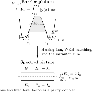
A localized state leaks through the forbidden interval between the inner turning points. Herring flux, WKB matching, and instanton calculus are different ways to determine the same low-energy coupling $J$. Diagonalizing the doublet gives $\Delta E=2J$.

What the Splitting Measures

Let

$$H = - \frac{\hbar^2}{2m} \frac{d^2}{dx^2} + V(x).$$

The symmetry condition is

$$V(-x)=V(x),$$

with two well-separated minima. The exact eigenfunctions have definite parity. For the lowest doublet, write

$$\begin{gathered} H\lvert e\rangle = E_e\lvert e\rangle, \qquad \mathsf P\lvert e\rangle = +\lvert e\rangle, \\ H\lvert o\rangle = E_o\lvert o\rangle, \qquad \mathsf P\lvert o\rangle = -\lvert o\rangle. \end{gathered}$$

In one dimension the nodeless even ground state lies below the odd state, so

$$\Delta E = E_o-E_e.$$

The mean doublet energy is

$$\bar E = \frac{E_e+E_o}{2}.$$

A useful two-state description requires a separation of scales. If $\delta_{\mathrm{intra}}$ is the gap from this doublet to the next pair of levels, then

$$\Delta E \ll \delta_{\mathrm{intra}}.$$

The inequality says more than “the barrier is high.” It ensures that left-right mixing can be discussed without simultaneously mixing several intrawell excitations.

Closed spectrum versus escape

All exact eigenvalues of a closed, self-adjoint double-well Hamiltonian are real. A wavepacket initially localized in one well can oscillate, dephase among several doublets, and recur, but it does not possess an intrinsic exponential decay width.

By contrast:

• open-barrier scattering asks for transmitted flux and gives a probability $T(E)$;
• a metastable well asks for a resonance width or decay rate $\gamma$;
• a symmetric bound double well asks for an energy splitting $\Delta E$.

The same forbidden-region action can appear in all three problems, but boundary conditions determine whether the exponential enters an amplitude, a probability, a splitting, or a rate.

Localized Basis and the Exact Doublet

Within the exact two-dimensional subspace, define

$$\begin{aligned} \lvert L\rangle &= \frac{ \lvert e\rangle+\lvert o\rangle }{\sqrt2}, \\ \lvert R\rangle &= \frac{ \lvert e\rangle-\lvert o\rangle }{\sqrt2}. \end{aligned}$$

These states are exactly orthonormal. They become spatially localized only when the parity partners have nearly identical probability densities within either well, as happens for a high barrier.

In this basis,

$$H_{\mathrm{eff}} = \begin{pmatrix} \bar E & -J\\ -J & \bar E \end{pmatrix}, \qquad J = \frac{\Delta E}{2}.$$

The sign of the off-diagonal entry is a phase convention chosen so that $J\gt0$ and the even state is lower. The spectral statement is invariant:

$$\Delta E=2J.$$

If the system begins in $\lvert L\rangle$ and remains within this doublet,

$$P_R(t) = \sin^2 \left( \frac{\Delta E\,t}{2\hbar} \right).$$

The first complete transfer occurs at

$$t_{\mathrm{transfer}} = \frac{\pi\hbar}{\Delta E}.$$

This dynamics is derived in the introductory Double-Well Potential page. Here the central task is to determine $J$ rather than assume it.

Nonorthogonal localized trial states

Localized trial functions constructed independently in the two wells generally overlap. Let

$$\begin{gathered} \langle \ell\vert\ell\rangle = \langle r\vert r\rangle = 1, \\ s \equiv \langle \ell\vert r\rangle, \qquad h \equiv \langle \ell\vert H\vert r\rangle, \\ E_d \equiv \langle \ell\vert H\vert\ell\rangle = \langle r\vert H\vert r\rangle, \end{gathered}$$

where phases have been chosen so that $s$ and $h$ are real. The normalized even and odd combinations are

$$\lvert \psi_\pm\rangle = \frac{ \lvert \ell\rangle \pm \lvert r\rangle }{ \sqrt{2(1\pm s)} }.$$

Their variational energies are

$$E_\pm = \frac{E_d\pm h}{1\pm s}.$$

Therefore

$$E_--E_+ = \frac{ 2(E_ds-h) }{ 1-s^2 }.$$

The effective coupling inferred from nonorthogonal trial states is

$$J_{\mathrm{eff}} = \frac{E_ds-h}{1-s^2}.$$

Only after orthogonalization, or when $s$ is negligible at the requested accuracy, may one identify $J$ with $-h$. Because $s$ and $h/E_d$ can carry the same tunneling exponential, dropping overlap in one place but not the other can corrupt the leading prefactor.

Herring Flux Formula

For a smooth symmetric one-dimensional well, the splitting can be extracted from one localized wavefunction without matching solutions through all four turning points.

Let $\psi_R(x)$ be a real approximate solution at energy $E_{\mathrm{loc}}$ that is localized in the right well, decays through the central barrier, and is normalized by

$$\int_0^\infty |\psi_R(x)|^2\,dx \simeq 1.$$

Then the leading splitting is

$$\Delta E \simeq \frac{2\hbar^2}{m} \psi_R(0)\psi_R'(0).$$

For a right-localized nodeless state, $\psi_R(0)\gt0$ and $\psi_R'(0)\gt0$. The formula measures probability-current capacity across the dividing point, even though each real stationary state separately carries no net current.

Wronskian derivation

Let $u_e$ and $u_o$ be the exact normalized even and odd eigenfunctions. Subtracting their Schrödinger equations after cross multiplication gives

$$\begin{aligned} \Delta E \int_0^\infty u_eu_o\,dx &= \frac{\hbar^2}{2m} \\ &\quad\times u_e(0)u_o'(0). \end{aligned}$$

The boundary terms at infinity vanish, while

$$u_e'(0)=0, \qquad u_o(0)=0.$$

In the high-barrier limit,

$$\int_0^\infty u_eu_o\,dx \simeq \frac12.$$

Moreover,

$$\begin{aligned} u_e(0) &\simeq \sqrt2\,\psi_R(0), \\ u_o'(0) &\simeq \sqrt2\,\psi_R'(0). \end{aligned}$$

Substitution yields Herring’s formula. Its usefulness is conceptual as well as computational: the spectral splitting is linear in a tunneling amplitude measured at the barrier, not quadratic like a transmission probability.

The formula assumes an isolated nearly degenerate doublet and reflection symmetry. Multidimensional versions replace the midpoint expression by a flux integral over a dividing surface, but then the tunneling path, transverse fluctuations, and coordinate-dependent mass metric require separate control.

WKB View

Let $E_n$ be the energy of the $n$th state localized in either isolated well. If $x_1(E_n)$ and $x_2(E_n)$ are the inner turning points bounding the forbidden interval, define the one-way barrier action

$$W_n = \int_{x_1(E_n)}^{x_2(E_n)} dx\, \sqrt{ 2m[V(x)-E_n] }.$$

In the semiclassical regime,

$$\frac{W_n}{\hbar}\gg1,$$

and the splitting has the structure

$$\Delta E_n \sim A_n e^{-W_n/\hbar}.$$

Here $A_n$ has dimensions of energy and is algebraic rather than exponential in the semiclassical parameter. It is often of order $\hbar\omega_{\mathrm{well}}$, but its numerical coefficient is not universal.

Exponential accuracy and prefactor accuracy

At exponential accuracy, the claim is only that

$$- \hbar \log \left( \frac{\Delta E_n}{E_{\mathrm{ref}}} \right) \sim W_n,$$

where $E_{\mathrm{ref}}$ is an energy scale with no tunneling exponential. This level of accuracy is robust and often physically sufficient.

A normalized asymptotic formula for $\Delta E_n$ requires the prefactor. For the lowest doublet, ordinary linear-turning-point connection formulas combined with a naive harmonic “attempt frequency” can miss an order-one coefficient. Controlled matching to the quadratic well bottom, a Herring calculation, or a correctly normalized instanton determinant resolves that issue.

This is why two statements must not be conflated:

1. WKB correctly identifies the barrier exponential.
2. Every compact textbook prefactor is automatically correct for the ground doublet.

The first is standard. The second is false without specifying the matching scheme and asymptotic regime.

Why transmission has twice the exponent

Across the barrier, a one-way wave amplitude scales as

$$t_{\mathrm{barrier}} \sim e^{-W_n/\hbar}.$$

A scattering probability squares that amplitude:

$$T \sim e^{-2W_n/\hbar}.$$

The bound-state splitting is linear in the off-diagonal amplitude:

$$\Delta E_n \sim e^{-W_n/\hbar}.$$

Importing the scattering-probability exponent into a splitting formula therefore produces an erroneous factor of two. Barrier Penetration and Tunneling is the canonical home for the scattering calculation.

Instanton View

Normalize the degenerate minima to

$$V(\pm a)=0.$$

The Euclidean instanton connecting $-a$ to $+a$ has action

$$S_0 = \int_{-a}^{a} dx\, \sqrt{2mV(x)}.$$

This is the zero-reference-energy version of the same geometric barrier action. The explicit quartic solution and its action are derived in Instantons in Quantum Mechanics Preview.

Define the one-dimensional fluctuation operators

$$\begin{aligned} \mathscr L_I &= - \frac{d^2}{d\tau^2} + \frac{1}{m} V''(x_I), \\ \mathscr L_0 &= - \frac{d^2}{d\tau^2} + \omega^2. \end{aligned}$$

At one loop, the one-instanton density can be written schematically as

$$\mathcal K_1 = \left( \frac{S_0}{2\pi\hbar} \right)^{1/2} \left[ \frac{ \det\mathscr L_0 }{ \det{}'\mathscr L_I } \right]^{1/2}.$$

The prime removes the translation zero mode. With consistent boundary conditions and determinant normalization, $\mathcal K_1$ has units of inverse time.

From an instanton gas to an energy doublet

Let

$$\zeta \equiv \mathcal K_1 e^{-S_0/\hbar}.$$

In a dilute gas, paths beginning and ending in the same well contain an even number of transitions, while paths ending in the opposite well contain an odd number. Summing those sectors gives

$$\begin{aligned} Z_{LL}(T) &\simeq \mathcal N e^{-E_{\mathrm{pert}}T/\hbar} \cosh(\zeta T), \\ Z_{RL}(T) &\simeq \mathcal N e^{-E_{\mathrm{pert}}T/\hbar} \sinh(\zeta T). \end{aligned}$$

Using

$$\cosh(\zeta T) = \frac12 \left( e^{\zeta T} + e^{-\zeta T} \right),$$

one reads off

$$\begin{aligned} E_e &= E_{\mathrm{pert}} - \hbar\zeta, \\ E_o &= E_{\mathrm{pert}} + \hbar\zeta. \end{aligned}$$

Thus

$$\Delta E = 2\hbar\mathcal K_1 e^{-S_0/\hbar}.$$

The factor of two is now transparent: one instanton determines the off-diagonal coupling

$$J = \hbar\mathcal K_1 e^{-S_0/\hbar},$$

and diagonalizing the two-state Hamiltonian gives $\Delta E=2J$.

Matching WKB and instantons

For the ground doublet, WKB naturally uses the turning-point action at $E_{\mathrm{loc}}\simeq\hbar\omega/2$, whereas the zero-energy instanton uses $S_0$. Since $E_{\mathrm{loc}}=O(\hbar)$, shifting the action to zero energy changes terms that can migrate between the exponent and prefactor.

Consequently:

• at leading exponential order, WKB and the instanton give the same suppression;
• at prefactor accuracy, endpoint matching and determinant normalization must be compared in the same convention;
• substituting $E=0$ into one formula while retaining the prefactor from another is not a controlled hybrid.

Correctly executed WKB and instanton calculations agree. Fluctuation Determinants Preview explains why that agreement is technically subtler than matching the actions alone.

Five Views of One Quantity

View	Primary input	Quantity computed	Main caveat
Exact spectrum	Full Hamiltonian and boundary conditions	$\Delta E=E_o-E_e$	Subtractive loss when the gap is extremely small
Effective doublet	Orthonormal localized basis	$\Delta E=2J$	$J$ is an input until derived microscopically
Herring flux	One normalized localized barrier tail	Midpoint flux and $\Delta E$	Requires an isolated nearly symmetric doublet
WKB	Turning points and forbidden action $W_n$	Exponential and, with matching, prefactor	Ground-state prefactors need quadratic-well matching
Instanton gas	Euclidean saddle, zero mode, determinant	$J$ and the parity doublet	Requires a valid dilute sector sum and normalized measure

These are not competing explanations. They are different projections of the same spectral problem:

$$\boxed{ \text{barrier leakage} \longrightarrow J \longrightarrow \Delta E=2J }$$

The box is useful here because it is the organizing identity of the page; most intermediate formulas are not boxed.

Exponential Sensitivity

Suppose a control parameter $\lambda$ changes the action and prefactor:

$$\Delta E(\lambda) = A(\lambda) \exp \left[ - \frac{S(\lambda)}{\hbar} \right].$$

Then

$$\frac{d\log\Delta E}{d\lambda} = \frac{d\log A}{d\lambda} - \frac{1}{\hbar} \frac{dS}{d\lambda}.$$

When $S/\hbar\gg1$, a modest fractional change in barrier height, width, or effective mass can change the splitting by orders of magnitude.

Mass and isotope dependence

If the potential and tunneling path are held fixed,

$$S \propto \sqrt m.$$

Therefore

$$\frac{d\log\Delta E}{d\log m} = \frac{d\log A}{d\log m} - \frac{S}{2\hbar}.$$

The action term normally dominates. This explains the strong isotope dependence of molecular tunneling splittings. In a real polyatomic molecule, isotopic substitution can also alter normal-mode coupling, zero-point energies, and the effective multidimensional path, so a one-coordinate $\sqrt m$ law is a diagnostic rather than a universal exact formula.

Tiny bias, large localization

Let a symmetry-breaking bias produce localized energies differing by $\varepsilon=E_L-E_R$. In an orthonormal basis,

$$H_{\mathrm{eff}} = \begin{pmatrix} \bar E+\varepsilon/2 & -J\\ -J & \bar E-\varepsilon/2 \end{pmatrix}.$$

The level gap is

$$\Delta E_{\mathrm{gap}} = \sqrt{ \varepsilon^2+4J^2 }.$$

At resonance, $\varepsilon=0$, the minimum gap is $2J$. If

$$|\varepsilon|\gg2J,$$

the eigenstates are mostly localized even when $|\varepsilon|$ is tiny compared with the intrawell scale. An algebraically small perturbation can therefore dominate an exponentially small tunneling matrix element. The full mixing-angle and avoided-crossing analysis belongs to Coupled Wells and Avoided Crossings.

This sensitivity does not constitute spontaneous symmetry breaking in a finite one-particle system. At exact symmetry and finite barrier, the nondegenerate ground state remains even. Localization arises from state preparation, bias, measurement, environmental coupling, or a limiting procedure in which the splitting tends to zero.

Extracting a Splitting Reliably

Symmetry-resolved diagonalization

For a symmetric numerical Hamiltonian:

1. diagonalize even and odd parity sectors separately;
2. pair states by energy, nodal structure, and localization within each well;
3. compute $\Delta E_n=E_{n,o}-E_{n,e}$;
4. verify that $\Delta E_n\ll\delta_{\mathrm{intra}}$;
5. increase the spatial domain, barrier resolution, and basis size;
6. compare $-\log\Delta E_n$ with the semiclassical action.

Separate parity sectors prevent an eigensolver from returning arbitrary rotations within a nearly degenerate numerical subspace. They do not remove floating-point cancellation in $E_{n,o}-E_{n,e}$; sufficiently small gaps require higher precision or an alternative flux or kernel extraction.

Euclidean kernel ratio

Within the isolated symmetric doublet,

$$\frac{Z_{RL}(T)}{Z_{LL}(T)} \simeq \tanh \left( \frac{\Delta E\,T}{2\hbar} \right).$$

Hence

$$\Delta E \simeq \frac{2\hbar}{T} \operatorname{artanh} \left[ \frac{Z_{RL}(T)}{Z_{LL}(T)} \right].$$

There is a useful Euclidean-time window:

$$\frac{\hbar}{\delta_{\mathrm{intra}}} \ll T \lesssim \frac{\hbar}{\Delta E}.$$

The first inequality suppresses higher intrawell states. The second avoids driving the ratio exponentially close to one, where extraction of $\Delta E$ becomes ill-conditioned. Euclidean Time and Imaginary-Time Action develops this separation of projection and resolution timescales.

Exactly solvable and numerical benchmarks

Double Delta Potential supplies an exact transcendental benchmark in which the even and odd binding momenta can be compared directly. For smooth wells, a robust validation sequence is:

$$\begin{gathered} \text{exact numerical spectrum} \\ \longleftrightarrow \text{Herring flux from a localized state} \\ \longleftrightarrow \text{WKB or instanton asymptotics}. \end{gathered}$$

Agreement of the exponent is a weaker test than agreement of the prefactor. Always state which one has been checked.

Double-Well Instanton Numerical Check implements this hierarchy for the quartic well, including parity blocks, basis-scale variation, a finite-difference cross-check, and a documented floating-point stopping point.

Applications and Limits

Molecular inversion

In ammonia, the two localized configurations correspond approximately to the nitrogen atom lying on opposite sides of the hydrogen plane. Tunneling produces inversion parity doublets visible in microwave and rovibrational spectroscopy. Isotopic substitution changes the effective masses and can strongly change the splitting.

The literal molecular problem is multidimensional: rotations, vibrations, and the inversion coordinate couple. A one-dimensional double well captures the origin of the doublet but not precision spectroscopy by itself.

Superconducting flux circuits

In a persistent-current flux qubit, two low-energy circuit configurations carry currents in opposite directions. Magnetic flux controls their bias, while quantum tunneling through an effective circuit potential produces the minimum avoided-crossing gap.

The two-level Hamiltonian is genuinely useful, but the tunneling coordinate is a collective circuit degree of freedom rather than the position of one particle. Capacitance supplies the kinetic metric, Josephson energies shape the potential, and environmental noise limits coherent dynamics. A spectral gap may remain well defined even when dephasing prevents observation of many left-right oscillations.

Molecular conformers, proton transfer, and engineered wells

The same structure appears in molecular conformations, hydrogen-transfer coordinates, semiconductor double wells, cold-atom double wells, and large-spin tunneling. Several qualifications can become decisive:

• more than one tunneling path may contribute;
• transverse zero-point energies modify the effective action;
• Berry phases can make amplitudes interfere rather than simply add;
• interactions can invalidate a one-particle two-state description;
• dissipation can renormalize the tunneling coupling and destroy coherent oscillations.

The reusable statement is not a universal prefactor. It is the chain from localized configurations to an off-diagonal amplitude and then to a spectral splitting.

Reliability Checklist

Before quoting a tunneling splitting, check:

1. Observable: Is the target a bound-state energy difference rather than a transmission probability or resonance width?
2. Doublet isolation: Is $\Delta E\ll\delta_{\mathrm{intra}}$?
3. Symmetry and bias: Are the wells truly degenerate to accuracy comparable with $J$?
4. Basis: Were localized trial states orthogonalized, or was their overlap retained?
5. Action: Are the turning points and reference energy appropriate to the state being split?
6. Prefactor claim: Is the result exponential-only, one-loop, or numerically normalized?
7. Instanton sectors: Does the observable require even, odd, or both transition-number sectors?
8. Numerics: Can the method resolve the exponentially small difference without subtractive loss?
9. Applications: Are multidimensional paths, interactions, and environmental decoherence negligible at the claimed accuracy?

Common Mistakes

• Calling $\Delta E$ a tunneling probability.
• Squaring the WKB amplitude and using $e^{-2W/\hbar}$ for a bound-state splitting.
• Confusing the off-diagonal coupling $J$ with the full symmetric splitting $2J$.
• Setting $J=-\langle\ell\vert H\vert r\rangle$ while ignoring nonzero overlap $s$.
• Treating localized states as exact stationary states at finite tunneling.
• Using the zero-energy instanton action with an unrelated WKB prefactor.
• Calling the gap away from resonance a pure tunneling splitting when bias dominates it.
• Subtracting two double-precision eigenvalues after their difference has fallen below numerical resolution.
• Inferring coherent oscillations from a spectral splitting without comparing the tunneling time with dephasing and leakage times.

Exercises

1. Recover the effective Hamiltonian

Starting from exact parity states $\lvert e\rangle$ and $\lvert o\rangle$, construct $\lvert L\rangle$ and $\lvert R\rangle$. Show that the off-diagonal matrix element is $-\Delta E/2$ and derive $P_R(t)$ for an initial left-localized state.

Solution

Define

$$\lvert L\rangle = \frac{\lvert e\rangle+\lvert o\rangle}{\sqrt2}, \qquad \lvert R\rangle = \frac{\lvert e\rangle-\lvert o\rangle}{\sqrt2}.$$

Then

$$\begin{aligned} \langle L\vert H\vert L\rangle &= \langle R\vert H\vert R\rangle = \frac{E_e+E_o}{2} = \bar E, \\ \langle L\vert H\vert R\rangle &= \frac{E_e-E_o}{2} = - \frac{\Delta E}{2}. \end{aligned}$$

Thus $J=\Delta E/2$. Expanding the initial state in parity eigenstates gives

$$\lvert\psi(t)\rangle = \frac{ e^{-iE_et/\hbar}\lvert e\rangle + e^{-iE_ot/\hbar}\lvert o\rangle }{\sqrt2}.$$

Projection onto $\lvert R\rangle$ yields

$$P_R(t) = \sin^2 \left( \frac{\Delta E\,t}{2\hbar} \right).$$

2. Retain localized-state overlap

For real normalized trial states with overlap $s$, diagonal energy $E_d$, and off-diagonal matrix element $h$, derive the even and odd variational energies and the effective coupling.

Solution

The normalized combinations are

$$\lvert\psi_\pm\rangle = \frac{ \lvert\ell\rangle\pm\lvert r\rangle }{ \sqrt{2(1\pm s)} }.$$

Their expectation values are

$$E_\pm = \frac{ 2E_d\pm2h }{ 2(1\pm s) } = \frac{E_d\pm h}{1\pm s}.$$

Therefore

$$\begin{aligned} E_--E_+ &= \frac{E_d-h}{1-s} - \frac{E_d+h}{1+s} \\ &= \frac{2(E_ds-h)}{1-s^2}. \end{aligned}$$

Identifying the splitting with $2J_{\mathrm{eff}}$ gives

$$J_{\mathrm{eff}} = \frac{E_ds-h}{1-s^2}.$$

3. Derive Herring’s midpoint formula

Starting from

$$Hu_e=E_eu_e, \qquad Hu_o=E_ou_o,$$

derive the Wronskian identity on $x\geq0$ and obtain the midpoint formula in the high-barrier limit.

Solution

Multiply the even equation by $u_o$, the odd equation by $u_e$, subtract, and integrate:

$$\begin{aligned} \Delta E \int_0^\infty u_eu_o\,dx &= \frac{\hbar^2}{2m} \\ &\quad\times \left[ u_eu_o' - u_ou_e' \right]_{x=0}. \end{aligned}$$

Decay removes the boundary term at infinity. Parity gives

$$u_o(0)=0, \qquad u_e'(0)=0,$$

so

$$\begin{aligned} \Delta E \int_0^\infty u_eu_o\,dx &= \frac{\hbar^2}{2m} \\ &\quad\times u_e(0)u_o'(0). \end{aligned}$$

For a well-isolated doublet,

$$\int_0^\infty u_eu_o\,dx\simeq\frac12,$$

and the right-localized function obeys

$$\begin{aligned} u_e(0) &\simeq \sqrt2\,\psi_R(0), \\ u_o'(0) &\simeq \sqrt2\,\psi_R'(0). \end{aligned}$$

Hence

$$\Delta E \simeq \frac{2\hbar^2}{m} \psi_R(0)\psi_R'(0).$$

4. Explain the WKB factor of two

The one-way forbidden action is $W$. Explain why a transmission probability scales as $e^{-2W/\hbar}$ while a tunneling splitting scales as $e^{-W/\hbar}$.

Solution

The decaying barrier tail gives an amplitude proportional to

$$e^{-W/\hbar}.$$

A transmission probability is a flux ratio quadratic in that amplitude, so

$$T\sim e^{-2W/\hbar}.$$

The double-well splitting is linear in the off-diagonal matrix element $J$, and $J$ is itself a tunneling amplitude:

$$J\sim e^{-W/\hbar}, \qquad \Delta E=2J.$$

Thus the splitting retains the one-way exponent.

5. Read the splitting from the instanton gas

Suppose

$$\begin{aligned} Z_{LL} &\propto e^{-E_{\mathrm{pert}}T/\hbar} \cosh(\zeta T), \\ Z_{RL} &\propto e^{-E_{\mathrm{pert}}T/\hbar} \sinh(\zeta T). \end{aligned}$$

Find the two energies and their splitting.

Solution

Using

$$\cosh(\zeta T) = \frac12 \left( e^{\zeta T} + e^{-\zeta T} \right),$$

the same-well kernel is a sum of two exponentials:

$$\begin{aligned} Z_{LL} &\propto \frac12 \Big[ e^{-(E_{\mathrm{pert}}-\hbar\zeta)T/\hbar} \\ &\qquad+ e^{-(E_{\mathrm{pert}}+\hbar\zeta)T/\hbar} \Big]. \end{aligned}$$

Therefore

$$E_e = E_{\mathrm{pert}}-\hbar\zeta, \qquad E_o = E_{\mathrm{pert}}+\hbar\zeta,$$

and

$$\Delta E=2\hbar\zeta.$$

For $\zeta=\mathcal K_1e^{-S_0/\hbar}$, this is the one-instanton splitting formula.

6. Estimate an isotope effect

Assume the potential and path are fixed, the prefactor change is negligible, and $S(m)=C\sqrt m$. If $m_2=\alpha m_1$, estimate $\Delta E(m_2)/\Delta E(m_1)$.

Solution

Since

$$S(m_2) = \sqrt\alpha\,S(m_1),$$

the ratio is

$$\frac{\Delta E(m_2)}{\Delta E(m_1)} \simeq \exp \left[ - \left( \sqrt\alpha-1 \right) \frac{S(m_1)}{\hbar} \right].$$

Even when $\alpha$ is of order unity, the ratio can be extremely small if $S(m_1)/\hbar\gg1$. In a molecule this estimate must be amended if isotope substitution changes the multidimensional path or transverse zero-point energies.

Cross-Links

• Instantons, Tunneling, and Nonperturbative Effects
• Double-Well Tunneling
• Barrier Penetration and Tunneling
• Euclidean Time and Imaginary-Time Action
• Instantons in Quantum Mechanics
• Fluctuation Determinants Preview
• Asymptotic Series and Nonperturbative Corrections
• Double-Well Potential
• Double Delta Potential
• Coupled Wells and Avoided Crossings
• Small Parameters and Error Estimates

References

1. A. Garg, “Tunnel Splittings for One-Dimensional Potential Wells Revisited”, American Journal of Physics 68, 430–437 (2000). Careful Herring, WKB, and instanton comparison, including the ground-state prefactor caveat.
2. S. Coleman, “The Uses of Instantons”, in Aspects of Symmetry, Cambridge University Press, 1985, pp. 265–350. Canonical derivation of the instanton gas, zero-mode measure, and double-well splitting.
3. C. Herring, “Critique of the Heitler–London Method of Calculating Spin Couplings at Large Distances”, Reviews of Modern Physics 34, 631–645 (1962). Source of the flux-surface method underlying the one-dimensional midpoint formula.
4. L. D. Landau and E. M. Lifshitz, Quantum Mechanics: Non-Relativistic Theory, 3rd ed., Pergamon, 1977, §50. Classic WKB treatment of nearly degenerate levels and barrier penetration.
5. B. Simon, “Semiclassical Analysis of Low Lying Eigenvalues. II. Tunnelling”, Annals of Mathematics 120, 89–118 (1984). Rigorous leading exponential asymptotics for multiwell spectral splittings.
6. B. Simon, “Semiclassical Analysis of Low Lying Eigenvalues. IV. The Flea on the Elephant”, Journal of Functional Analysis 63, 123–136 (1985). Analysis of how tiny asymmetries compete with exponentially small double-well splittings.
7. M. V. Berry and K. E. Mount, “Semiclassical Approximations in Wave Mechanics”, Reports on Progress in Physics 35, 315–397 (1972). Uniform approximations, connection methods, and the scope of semiclassical wave mechanics.
8. B. R. Holstein and A. R. Swift, “Path Integrals and the WKB Approximation”, American Journal of Physics 50, 829–832 (1982). Direct bridge between semiclassical path integrals and WKB.
9. F. B. Brown, S. C. Tucker, and D. G. Truhlar, “Semiclassical Reaction-Path Methods Applied to Calculate the Tunneling Splitting in Ammonia”, Journal of Chemical Physics 83, 4451–4455 (1985). Molecular inversion example and multidimensional reaction-path corrections.
10. T. P. Orlando et al., “Superconducting Persistent-Current Qubit”, Physical Review B 60, 15398–15413 (1999). Effective double-well and avoided-crossing structure in a superconducting circuit.
11. J. Zinn-Justin, Path Integrals in Quantum Mechanics, Oxford University Press, 2005. Detailed treatment of instantons, multi-instanton sectors, and nonperturbative level splittings.