Double-Well Instanton Numerical Check

An instanton prediction is not adequately tested by finding a straight line on a logarithmic plot. This notebook compares the lowest even–odd splitting of a fixed quartic double well with two semiclassical formulas, resolves the doublet in parity sectors, varies the basis dimension and scale, and repeats two representative calculations with an independent finite-difference method.

Across $0.30\ge g\ge0.06$, the numerical gap falls from $2.95\times10^{-2}$ to $3.33\times10^{-10}$. The finite-energy WKB ratio to the numerical gap improves from $1.378$ to $0.9946$, while the one-loop instanton ratio improves from $1.391$ to $1.0479$. Those ratios test more than the shared exponential: they also expose how finite-energy endpoint effects and loop corrections are allocated between exponent and prefactor.

At the smallest retained coupling, changing the basis dimension and oscillator scale changes the gap by about $5.5\times10^{-6}$ relative. That is a numerical floor, not evidence for six more asymptotic digits. The calculation stops there deliberately.

Run the investigation. The program and retained results below support the stated experiment. Follow Running an Experiment for environment and output-directory guidance. The recorded evidence applies to its stated parameters and environment.

Canonical Boundaries

This page owns the numerical experiment and its retained artifacts. It does not replace the analytic pages.

Object	Canonical home	Role here
parity doublets and localized states	Double-Well Potential	physical first encounter
smooth-well tunneling model	Double-Well Tunneling	model interpretation
Herring, WKB, instanton, and spectral dictionary	Tunneling Splittings	general method
Euclidean saddle and action	Instantons in Quantum Mechanics	instanton derivation
convention-complete quartic calculation	Double-Well Splitting	hand-worked benchmark
reusable code, sweeps, convergence, and independent discretization	this page	computational evidence

The formulas below are repeated only to define the program’s inputs and outputs. Follow the canonical pages for their derivations.

Physical Problem

The dimensionless Hamiltonian is

$$\begin{aligned} H_g &= -\frac{g^2}{2} \frac{d^2}{dq^2} + U(q), \\ U(q) &= \frac12 \left( q^2-1 \right)^2. \end{aligned}$$

The minima lie at $q=\pm1$, the barrier height is $U(0)=1/2$, and the harmonic frequency in either well is $\omega_0=2$. The effective Planck constant is $g$, so the semiclassical regime is $g\ll1$.

Let $\epsilon_e$ and $\epsilon_o$ be the lowest even and odd eigenvalues. The observable is the closed-system spectral gap

$$\Delta\epsilon \equiv \epsilon_o-\epsilon_e \gt0.$$

It is neither a transmission probability nor a decay width. The corresponding left–right coupling is $J=\Delta\epsilon/2$.

Analytic Benchmarks

Finite-energy WKB

Using the leading local ground energy $\epsilon_{\mathrm{loc}}=g$, the inner turning point is

$$q_t(g) = \sqrt{ 1-\sqrt{2g} }.$$

The one-way forbidden action is

$$\begin{aligned} W(g) &= 2 \int_0^{q_t} \sqrt{ \left( 1-q^2 \right)^2 - 2g } \,dq, \\ \Delta\epsilon_{\mathrm{WKB}} &= \frac{2g}{\pi} \exp \left[ -\frac{W(g)}{g} \right]. \end{aligned}$$

The program evaluates $W(g)$ with 512-point Gauss–Legendre quadrature and repeats it at order 256. The largest action change in the retained sweep is $8.21\times10^{-9}$.

One-loop instanton

The zero-energy Euclidean trajectory is $q_I(s)=\tanh(s-s_0)$, and its action is

$$S_0 = \int_{-1}^{1} \sqrt{2U(q)} \,dq = \frac43.$$

For this Hamiltonian convention, the one-loop splitting is

$$\Delta\epsilon_{\mathrm{inst}} = 4 \sqrt{ \frac{8g}{\pi} } \exp \left( -\frac{4}{3g} \right) \left[ 1+O(g) \right].$$

The $O(g)$ reminder is part of the prediction. A ratio that differs from one by several percent at finite $g$ is compatible with the stated approximation.

Exponent and prefactor diagnostics

To inspect the exponent without pretending the prefactor is constant, define

$$S_{\mathrm{eff}}(g) \equiv -g \log \left( \frac{ \Delta\epsilon_{\mathrm{num}} }{ \sqrt g } \right).$$

If

$$\Delta\epsilon \sim C\sqrt g\, e^{-S_0/g},$$

then

$$S_{\mathrm{eff}}(g) = S_0-g\log C+O(g^2).$$

The complementary prefactor diagnostic is

$$C_{\mathrm{eff}}(g) \equiv \frac{ \Delta\epsilon_{\mathrm{num}} e^{S_0/g} }{ \sqrt g }.$$

The one-loop limit is $C=4\sqrt{8/\pi}=6.383\ldots$. In the retained data, $C_{\mathrm{eff}}$ rises from $4.589$ at $g=0.30$ to $6.091$ at $g=0.06$.

Production Spectrum

Oscillator representation

Use harmonic-oscillator states with adjustable frequency $\Omega$. In that basis,

$$q = \sqrt{ \frac{g}{2\Omega} } \left( a+a^\dagger \right),$$

and the projected Hamiltonian is assembled as

$$\begin{aligned} H_g &= H_{\Omega} + \frac12q^4 \\ &\quad- \left( 1+\frac{\Omega^2}{2} \right)q^2 + \frac12I, \\ H_{\Omega} &= g\Omega \left( N+\frac12 \right). \end{aligned}$$

The code constructs four guard states beyond the retained dimension before projecting $q^4$. This prevents the top edge of a prematurely truncated position matrix from corrupting exact polynomial matrix elements.

Resolve parity before diagonalization

Because $U(-q)=U(q)$, oscillator states of even and odd index do not mix. The program diagonalizes

$$\begin{aligned} H^{(e)}_{jk} &= \langle 2j|H_g|2k\rangle, \\ H^{(o)}_{jk} &= \langle 2j+1|H_g|2k+1\rangle \end{aligned}$$

separately. This prevents a generic eigensolver from returning arbitrary rotations of a nearly degenerate pair and provides an exact structural check: the computed cross-parity block vanishes.

Parity resolution does not eliminate subtraction error. The gap still comes from two numbers of order $g$ whose difference can be many orders of magnitude smaller.

Production controls

The retained sweep uses

$$\begin{gathered} N=220, \qquad \Omega=2, \\ 0.06\le g\le0.30. \end{gathered}$$

Each gap is compared with $N=160$ and with $\Omega=1.5,3$ at $N=220$. The next state above the doublet is also retained so that the isolation ratio

$$r_{\mathrm{iso}} = \frac{ \Delta\epsilon }{ \epsilon_2- (\epsilon_e+\epsilon_o)/2 }$$

can be checked directly.

Parameter Sweep

Selected rows are shown below; the downloadable table contains all ten couplings.

$g$	$\Delta\epsilon_{\mathrm{num}}$	WKB / numerical	instanton / numerical	$S_{\mathrm{eff}}$
$0.30$	$2.95206\times10^{-2}$	$1.3775$	$1.3908$	$0.8762$
$0.20$	$3.01756\times10^{-3}$	$1.1747$	$1.2039$	$0.9997$
$0.15$	$2.99603\times10^{-4}$	$1.1008$	$1.1380$	$1.0747$
$0.10$	$3.01409\times10^{-6}$	$1.0389$	$1.0846$	$1.1561$
$0.08$	$9.78792\times10^{-8}$	$1.0163$	$1.0657$	$1.1901$
$0.06$	$3.33263\times10^{-10}$	$0.9946$	$1.0479$	$1.2249$

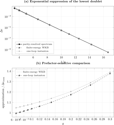
Top: parity-resolved gaps and the two semiclassical estimates over nearly eight orders of magnitude. Bottom: ratios to the numerical gap expose prefactor-level disagreement that a logarithmic gap plot largely hides. The finite-energy WKB curve crosses the numerical result between $g=0.07$ and $0.06$; this crossing is not evidence that its omitted corrections vanish.

Both approximations capture the exponential suppression. Their finite-$g$ behavior differs because the WKB formula retains the local energy inside $W(g)$, while the displayed instanton formula expands around the zero-energy action and organizes finite-$g$ effects as loop corrections.

Agreement of either ratio with one at a single coupling can therefore be accidental. The meaningful evidence is the controlled trend together with a numerical error estimate well below the approximation error.

Independent Finite-Difference Check

The second representation uses a centered grid on $-L<q<L$ with Dirichlet endpoints. For spacing $h$, the tridiagonal matrix has

$$\begin{aligned} d_j &= \frac{g^2}{h^2} + U(q_j), \\ e_j &= -\frac{g^2}{2h^2}. \end{aligned}$$

The two lowest eigenvalues are located by Sturm-sequence bisection; no dense grid matrix is formed. This implementation shares the Hamiltonian convention with the basis calculation but not its representation or eigensolver.

The centered second difference has $O(h^2)$ error. Consecutive grids therefore support the Richardson estimate

$$\Delta\epsilon_R(h) = \frac{ 4\Delta\epsilon(h) - \Delta\epsilon(2h) }{3}.$$

The retained half-width is $L=3$. At the finest grid, the extrapolated relative differences from the oscillator-basis result are $8.93\times10^{-10}$ at $g=0.15$ and $6.87\times10^{-7}$ at $g=0.08$.

Basis and Grid Convergence

At $g=0.06$, the reference in the convergence table is the median of nine high-resolution calculations using $N=160,220,280$ and $\Omega=1.5,2,3$:

$$\Delta\epsilon_{\mathrm{ref}} = 3.3326408\times10^{-10}.$$

The largest deviation among those nine values is $1.54\times10^{-15}$ in absolute energy, or $4.62\times10^{-6}$ relative to the gap.

$N$ at $\Omega=2$	computed gap	relative difference from the median
$40$	$-2.39025\times10^{-9}$	$8.17$
$60$	$3.33263\times10^{-10}$	$2.64\times10^{-6}$
$80$	$3.33262\times10^{-10}$	$5.41\times10^{-6}$
$120$	$3.33263\times10^{-10}$	$4.43\times10^{-6}$
$220$	$3.33263\times10^{-10}$	$4.62\times10^{-6}$
$280$	$3.33263\times10^{-10}$	$2.89\times10^{-6}$

The negative $N=40$ gap is not a physical parity inversion. The two truncated parity sectors have different variational errors, each much larger than the true splitting. Once the basis resolves both sectors, the gap reaches a plateau. Beyond that plateau, adding states does not produce monotone improvement because roundoff in the two eigenvalues is already comparable with the last reported digits of their difference.

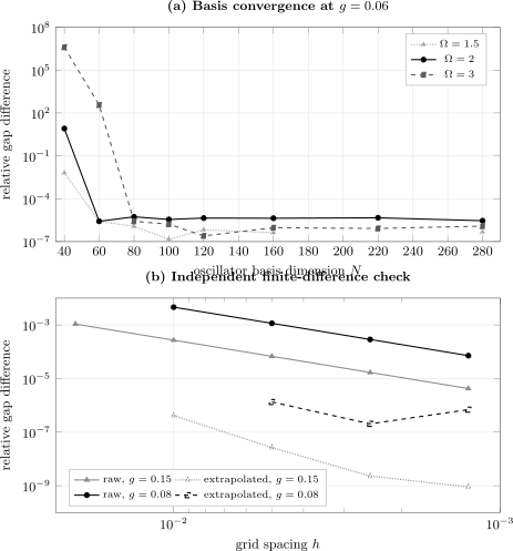
Top: at $g=0.06$, several oscillator scales converge to a relative plateau of a few parts in $10^6$; poor bases can even give the wrong parity ordering. Bottom: the independent centered finite difference displays second-order convergence, while Richardson extrapolation removes the leading $h^2$ error. Nonmonotonic extrapolated points at the finest grids mark the onset of subtraction and bisection roundoff.

Validation Ledger

Check	Retained value	What it tests
$g=0.15$ benchmark difference	$6.66\times10^{-13}$ relative	convention and matrix assembly
maximum Hermiticity defect	$5.68\times10^{-14}$	projected Hamiltonian construction
maximum cross-parity matrix element	$0$	symmetry block construction
maximum eigenpair residual	$7.02\times10^{-14}$	dense parity eigensolver
maximum WKB quadrature change	$8.21\times10^{-9}$ in action	forbidden-region integral
$g=0.08$ high-$N$ basis plateau	$1.25\times10^{-8}$ relative	basis and scale sensitivity
$g=0.06$ high-$N$ basis plateau	$4.62\times10^{-6}$ relative	roundoff-limited endpoint
finite difference at $g=0.15$	$8.93\times10^{-10}$ relative	independent representation
finite difference at $g=0.08$	$6.87\times10^{-7}$ relative	independent small-gap extraction
production gaps	positive and monotonically suppressed	parity order and parameter trend

Residuals and Hermiticity show that the represented matrices are solved accurately. They do not establish basis convergence. The $N$ and $\Omega$ sweep supplies that evidence. The finite-difference calculation then tests the same observable without the oscillator basis.

Error Budget at g = 0.08

At $g=0.08$,

$$\Delta\epsilon_{\mathrm{num}} = 9.7879224\times10^{-8}.$$

Source	Retained scale	Interpretation
WKB discrepancy	$1.63\times10^{-2}$ relative	finite-order physical approximation
one-loop instanton discrepancy	$6.57\times10^{-2}$ relative	omitted loop corrections
basis and scale variation	$1.13\times10^{-8}$ relative	production spectral uncertainty proxy
finite-difference extrapolation	$6.87\times10^{-7}$ relative	independent numerical check
WKB quadrature refinement	$8.10\times10^{-9}$ in $W$	integration error before division by $g$

The numerical discrepancies are several orders of magnitude below the approximation errors. The benchmark can therefore distinguish semiclassical physics from discretization error at this coupling.

At $g=0.06$, the physical comparison is still useful, but the relative basis spread has grown to $5.46\times10^{-6}$. Extending the sweep much further in ordinary double precision would require a different extraction strategy or higher precision.

Reproduce the Calculation

Run the downloaded program from the folder where you saved it:

python double-well-instanton-check.py --output-dir results

NumPy is the only required package. The optional —plot flag uses Matplotlib for quick-look PNGs; the documentation figures are generated from the linked pgfplots sources and retained CSVs.

Artifact	Contents
Python program	basis and finite-difference solvers, sweeps, validation, and export
semiclassical sweep	ten couplings, exact gaps, WKB actions, instanton estimates, ratios, and diagnostics
basis convergence	two small couplings, three oscillator scales, and eight basis dimensions
finite-difference convergence	raw and Richardson-extrapolated grid gaps
benchmark figure source	pgfplots source for the splitting comparison
convergence figure source	pgfplots source for basis and grid convergence

The program writes its runtime, Python version, NumPy version, platform, output paths, validation metrics, and final pass state. The retained reference run used Python 3.12.13 and NumPy 2.3.5 on 64-bit Windows.

Reproducibility metadata

Item	Retained setting
model	$H_g=-(g^2/2)d^2/dq^2+(q^2-1)^2/2$
production basis	harmonic oscillator, $N=220$, $\Omega=2$
basis refinements	$N=40$ through $280$; $\Omega=1.5,2,3$
WKB quadrature	Gauss–Legendre orders $512$ and $256$
finite-difference box	$-3<q<3$, Dirichlet endpoints
finite-difference solver	Sturm bisection, 96 iterations per eigenvalue
arithmetic	NumPy binary64
randomness	none
code license	MIT
data transformation	direct CSV export; no smoothing or fitted parameters

The $g$ range and convergence schedule are fixed in the source. No fit window is selected after inspecting the result.

Known Failure Modes

• Converged energies, unconverged gap. Absolute errors that are harmless for $\epsilon_e$ and $\epsilon_o$ can overwhelm their difference.
• Unresolved parity sectors. A generic full-matrix eigensolver may rotate a near-degenerate pair; an undersized parity basis may even reverse the computed ordering.
• Treating a residual as a continuum error bar. A small algebraic residual says nothing about basis dimension, oscillator scale, box size, or grid spacing.
• Pushing binary64 past its useful range. Once basis variation reaches the desired digits, a larger matrix may amplify roundoff rather than improve the gap.
• Confusing exponent and prefactor accuracy. Agreement on $S_0=4/3$ does not validate the one-loop normalization.
• Mixing the finite-energy and zero-energy organizations. Replacing $W(g)$ by $S_0$ while retaining the finite-energy WKB prefactor does not define a controlled next-order formula.
• Ignoring finite-box error. Grid refinement at fixed $L$ cannot reveal a domain that truncates the wavefunction tails.
• Calling the numerical result experimentally exact. It is a converged solution of the stated one-dimensional Hamiltonian, not a model-discrepancy assessment for a molecule or device.

Further Investigations

1. Repeat the parity calculation in arbitrary precision and determine where binary64 ceases to resolve the doublet.
2. Compute the determinant ratio with a Gel’fand–Yaglom method and test the one-loop prefactor directly.
3. Add a weak bias and compare the exact low-energy pair with the two-state avoided-crossing Hamiltonian.
4. Track excited-state doublets and test how the finite-energy WKB action changes with intrawell quantum number.
5. Extract the gap from an imaginary-time kernel ratio instead of spectral subtraction.
6. Compare the leading formulas with higher-order uniform WKB or resurgent corrections without fitting them to the retained data.

Exercises

1. Verify the parity blocks

Show from oscillator selection rules that $q^2$ and $q^4$ connect only states whose indices differ by an even integer. Explain why the Hamiltonian separates into even and odd blocks.

Solution

Since $q\propto a+a^\dagger$, one power of $q$ changes the oscillator index by an odd integer. An even power changes it by an even integer. Therefore

$$\langle n|q^2|m\rangle = \langle n|q^4|m\rangle = 0$$

when $n$ and $m$ have opposite parity. The oscillator Hamiltonian is diagonal, so every term in $H_g$ preserves parity. Ordering the basis as even indices followed by odd indices makes $H_g$ block diagonal.

2. Why can a variational calculation give a negative gap?

At $g=0.06$, the $N=40$, $\Omega=2$ calculation gives $\epsilon_o-\epsilon_e<0$. Does this contradict the theorem that the ground state of a one-dimensional confining potential is even and nodeless?

Solution

No. Rayleigh–Ritz gives an upper bound independently in each truncated parity subspace:

$$\epsilon_e^{(N)}\ge\epsilon_e, \qquad \epsilon_o^{(N)}\ge\epsilon_o.$$

It does not require the two upper-bound errors to be equal. If

$$\epsilon_e^{(N)}-\epsilon_e \gt \epsilon_o^{(N)}-\epsilon_o + \Delta\epsilon,$$

the truncated difference is negative even though the exact ordering is unchanged. The sign failure is a convergence diagnostic for the difference, not a physical parity inversion.

3. Derive the Richardson formula

Assume the grid gap has the expansion

$$\Delta(h) = \Delta_* + Ah^2 + Bh^4 + O(h^6).$$

Construct a combination of $\Delta(h)$ and $\Delta(2h)$ that cancels the $Ah^2$ term.

Solution

One has

$$\Delta(2h) = \Delta_* + 4Ah^2 + 16Bh^4 + O(h^6).$$

Therefore

$$\begin{aligned} \frac{ 4\Delta(h)-\Delta(2h) }{3} &= \Delta_* - 4Bh^4 \\ &\quad+ O(h^6). \end{aligned}$$

The leading second-order grid error is removed. This extrapolation is trustworthy only after the raw values have entered the $h^2$ regime.

4. Extract the leading action from two gaps

Neglect the variation of the prefactor and estimate $S_0$ from numerical gaps at $g_1=0.10$ and $g_2=0.08$ using

$$\Delta(g) \approx C\sqrt g\,e^{-S_0/g}.$$

Solution

Taking a ratio gives

$$S_0^{(12)} = - \frac{ \log \left[ \dfrac{\Delta(g_1)/\sqrt{g_1}} {\Delta(g_2)/\sqrt{g_2}} \right] }{ 1/g_1-1/g_2 }.$$

Using $\Delta(0.10)=3.0140910\times10^{-6}$ and $\Delta(0.08)=9.7879224\times10^{-8}$ gives

$$S_0^{(12)} \approx 1.326.$$

This is close to $4/3$, but the difference should not be interpreted as a numerical error: the prefactor has $O(g)$ corrections that the two-point estimate neglects.

5. Identify the dominant error at g = 0.08

Using the error-budget table, decide whether the comparison can distinguish the WKB and instanton discrepancies from numerical error.

Solution

The independent finite-difference difference, $6.87\times10^{-7}$ relative, is the largest listed numerical discrepancy. The WKB and instanton discrepancies are $1.63\times10^{-2}$ and $6.57\times10^{-2}$. Their ratios to the numerical scale are approximately

$$2.4\times10^4 \qquad\text{and}\qquad 9.6\times10^4.$$

Thus the numerical uncertainty is far below both physical approximation errors. The benchmark can resolve their difference comfortably.

6. Estimate the binary64 subtraction limit

Let each parity eigenvalue have absolute roundoff of order $\epsilon_{\mathrm{mach}}E$, with $E\sim g$ and $\epsilon_{\mathrm{mach}}\approx2.2\times10^{-16}$. Estimate the relative roundoff amplification in the gap at $g=0.06$.

Solution

The scale estimate is

$$\begin{aligned} \frac{ \epsilon_{\mathrm{mach}}g }{ \Delta\epsilon } &\sim \frac{ (2.2\times10^{-16})(0.06) }{ 3.33\times10^{-10} } \\ &\approx 4.0\times10^{-8}. \end{aligned}$$

This is a lower bound on practical sensitivity, because matrix conditioning, eigensolver operations, and basis cancellation add larger constants. The observed few-parts-in-$10^6$ plateau is therefore plausible. Resolving substantially smaller gaps calls for higher precision or an observable that avoids subtracting two nearly equal eigenvalues.

Cross-Links

• Computational Notebooks defines the convergence and reproducibility contract used here.
• Double-Well Splitting carries out the same convention-fixed calculation by hand.
• Tunneling Splittings explains why a spectral gap carries an amplitude exponent rather than a transmission-probability exponent.
• Instantons in Quantum Mechanics derives the finite-action Euclidean saddle.
• Fluctuation Determinants Preview explains the zero mode and one-loop prefactor.
• Barrier Penetration and Tunneling develops the WKB forbidden-region action.
• Matrix Diagonalization and Convergence Tests provide the reusable numerical methods.

References

1. L. D. Landau and E. M. Lifshitz, Quantum Mechanics: Non-Relativistic Theory, 3rd ed., §50, Pergamon Press (1977).
2. S. Coleman, Aspects of Symmetry, Chapter 7, Cambridge University Press (1985).
3. R. Rajaraman, Solitons and Instantons, Chapter 10, North-Holland (1982).
4. J. Zinn-Justin and U. D. Jentschura, “Multi-instantons and exact results I: Conjectures, WKB expansions, and instanton interactions,” Annals of Physics 313, 197–267 (2004), doi:10.1016/j.aop.2004.04.004.
5. J. Zinn-Justin and U. D. Jentschura, “Multi-instantons and exact results II: Specific cases, higher-order effects, and numerical calculations,” Annals of Physics 313, 269–325 (2004), doi:10.1016/j.aop.2004.04.003.
6. N. J. Higham, Accuracy and Stability of Numerical Algorithms, 2nd ed., SIAM (2002).
7. G. H. Golub and C. F. Van Loan, Matrix Computations, 4th ed., Johns Hopkins University Press (2013).