Reproducibility Benchmarks

A reproducible program is not merely one that runs twice. A trustworthy computational result needs a named observable, a physical or mathematical anchor, an explicit tolerance, independent invariants where possible, machine-readable evidence, and a statement of what a passing test does not establish.

This page defines a cross-notebook acceptance suite for the Computational AMO chapter. The retained run reports:

Benchmark group	Evidence status	Result	Headline anchor
hydrogen energies	analytic specification	$5/5$	$E_n=-1/(2n^2)E_{\mathrm h}$
variational helium	artifact verified	$6/6$	$\zeta_*=27/16$
minimal-basis $\mathrm{H}_2^+$	artifact verified	$7/7$	$E_g(2a_0)=-0.553771495318482E_{\mathrm h}$
coherent Rabi oscillations	artifact verified	$5/5$	resonant $\pi$ pulse gives $P_e=1$
optical Bloch steady state	artifact verified	$5/5$	$\rho_{ee}^{\mathrm{ss}}=1/3$ at $\Omega=\Gamma$
Jaynes–Cummings splitting	artifact verified	$5/5$	$\Delta E_n=2\hbar g\sqrt{n+1}$
Doppler force curve	artifact verified	$6/6$	red detuning damps near $v=0$
versioning and dependencies	artifact verified	$4/4$	all declared outputs, runtimes, licenses, and seeds

The suite therefore passes

$$43/43$$

top-level checks across eight groups. Six upstream notebook metadata files contribute another $104$ retained Boolean validations that are folded into their respective suite checks. Twelve primary CSV and JSON inputs receive byte counts and SHA-256 digests, while the six producer manifests account for $33$ declared output files.

Those numbers describe the retained evidence. They are not a probability that the models are true.

Canonical Scope

This page is the canonical home for:

• the cross-notebook acceptance contract;
• benchmark identifiers, observables, expected values, and tolerances;
• the distinction between analytic specifications and artifact-backed checks;
• the machine-readable report and compact summary;
• evidence hashing and runtime recording;
• dependency, schema, and benchmark-version policy;
• failure triage;
• rules for adding or changing a benchmark; and
• the limits of what reproducibility tests can claim.

The individual notebooks remain canonical for their physics, numerical methods, derivations, convergence studies, and model limitations:

• Radial Schrödinger Solvers owns radial boundary-value methods and the full hydrogenic benchmark ladder.
• Variational Helium Notebook owns the effective-charge trial calculation.
• Molecular Orbital Computation owns the minimal $\mathrm{H}_2^+$ generalized eigenproblem.
• Time-Dependent Two-Level Systems Notebook owns Rabi, pulse-area, Ramsey, and rotating-wave benchmarks.
• Optical Bloch Equation Notebook owns dissipative two-level transients and steady response.
• Cavity QED Simulation Notebook owns dressed doublets, vacuum exchange, cutoff studies, and loss.
• Laser Cooling Simulation Notebook owns Doppler force, friction, diffusion, temperature, and relaxation.

The suite samples and cross-checks those artifacts. It does not duplicate their complete calculations.

Reproducibility Contract

The executable suite uses only the Python standard library:

• Download the suite
• Machine-readable report
• Compact benchmark summary

From the repository root, run:

python public/notebooks/atoms-molecules-light/amo-reproducibility-benchmarks.py `
  --data-dir public/data/amo `
  --output-dir public/data/amo

The retained console summary is:

PASS hydrogen           5/5 checks
PASS helium             6/6 checks
PASS h2plus             7/7 checks
PASS rabi               5/5 checks
PASS optical_bloch      5/5 checks
PASS cavity_qed         5/5 checks
PASS doppler            6/6 checks
PASS infrastructure     4/4 checks
summary: 43/43 checks passed across 8 benchmark groups

The suite has no random seed because it performs no random sampling. It always writes the JSON report and CSV summary. If any check fails, the report records the failure, the failed identifiers are printed, and the process returns a nonzero status.

Run producers before the suite

The suite consumes retained artifacts; it does not silently regenerate them. The correct order is:

1. run an affected producer notebook;
2. inspect and accept its local validations;
3. regenerate the cross-notebook report;
4. review numerical, schema, and hash changes;
5. build the documentation site; and
6. commit the program, data, report, and explanatory page together.

Running only the suite against stale CSV files tests the stale files. Provenance begins with knowing what was actually executed.

Terms and Levels of Evidence

Different communities use “reproducibility” and “replicability” in different ways. The National Academies recommends distinguishing:

• computational reproducibility: obtaining consistent results from the same input data, computational steps, methods, code, and analysis conditions;
• replicability: obtaining consistent results in a new study that addresses the same scientific question with new data; and
• repeatability in metrology and engineering contexts: repeated measurement under tightly matched conditions.

For these notebooks, four evidence levels are useful.

Level 1: re-execution

The same program, inputs, dependencies, and environment produce the same named observables within tolerance. Bitwise equality can be tested when the pipeline is deterministic and serialization is controlled, but it is not the only acceptable criterion.

Level 2: independent implementation

A different algorithm or implementation recovers the same mathematical quantity. Examples include:

• analytic versus matrix Rabi propagation;
• analytic versus linear optical Bloch steady states;
• symmetry-adapted versus generalized $\mathrm{H}_2^+$ eigenvalues;
• analytic versus finite-difference Doppler friction; and
• finite-cutoff versus untruncated coherent-state sums in cavity QED.

This level is stronger than rerunning one code path because a single implementation mistake is less likely to be shared.

Level 3: model cross-check

Independent identities constrain the same result:

• norm, trace, positivity, and conserved excitation;
• generalized metric normalization;
• variational upper bounds and virial stationarity;
• parity, oddness, and sign reversal;
• convergence order and cutoff stability; and
• known limiting cases.

An invariant can still share assumptions with the main calculation. Its independence must be argued, not presumed.

Level 4: physical replication

An experiment or independent high-fidelity calculation tests whether the model predicts the physical system. The suite does not reach this level. A program can reproduce its own idealized curves perfectly while omitting the dominant experimental mechanism.

Evidence Pipeline

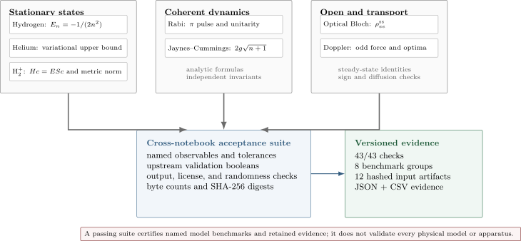
The suite combines analytic anchors, independent solvers, physical invariants, declared tolerances, upstream validations, runtime records, and artifact identities. A pass certifies the named model contracts and retained evidence. It does not certify every physical assumption or apparatus.

Anatomy of a Scientific Benchmark

A useful benchmark is more than an expected number.

Named quantity

The observable must identify:

• the Hamiltonian or evolution equation;
• state, symmetry sector, and initial condition;
• parameter values;
• units and frequency convention;
• basis or discretization;
• normalization convention; and
• any post-processing used to extract the number.

“Helium energy” is ambiguous. “The optimized one-parameter clamped-nucleus nonrelativistic helium trial energy in Hartree atomic units” is testable.

Independent oracle

An oracle can be:

• an exact analytic expression;
• a symmetry or conservation law;
• a variational inequality;
• a second algorithm;
• an asymptotic limit;
• a manufactured solution;
• a trusted reference dataset with provenance; or
• a controlled refinement limit.

The same formula copied into two functions is not an independent oracle.

Tolerance

Every floating-point check needs a tolerance tied to:

• the scale of the observable;
• expected discretization or integration error;
• conditioning;
• cancellation;
• the arithmetic used;
• upstream reference uncertainty; and
• the purpose of the test.

A tolerance should be tight enough to catch plausible regressions and loose enough to survive justified platform-level variation. It should not be chosen after looking at a failed result merely to make the test pass.

Failure message

A failed check should name:

• the benchmark;
• actual and expected values;
• tolerance;
• units;
• likely layer of failure; and
• evidence needed to decide whether the code, benchmark, or model changed.

The JSON report preserves those fields for every top-level check.

Claim boundary

Every benchmark group includes a sentence stating what it does not certify. This keeps a numerical pass from silently expanding into a physical claim.

Benchmark 1: Hydrogen Energies

For the infinite-mass nonrelativistic Coulomb Hamiltonian in Hartree atomic units,

$$E_n = -\frac{1}{2n^2}E_{\mathrm h}.$$

The suite records:

$$\begin{aligned} E_1&=-0.5E_{\mathrm h},\\ E_2&=-0.125E_{\mathrm h},\\ E_3&=-0.0555555555555556E_{\mathrm h}. \end{aligned}$$

It also requires:

$$E_{2s}=E_{2p}$$

for the ideal Coulomb Hamiltonian and checks that the bound levels approach zero from below.

Evidence status

This group is labeled analytic_specification, not artifact_verified. The suite recomputes and records exact targets, but it does not execute a retained radial grid solver. Claiming otherwise would confuse a benchmark definition with evidence that a discretization met it.

What a radial solver must add

A future artifact-backed hydrogen gate should require:

1. energy convergence under grid refinement;
2. independent box-size convergence;
3. correct radial node count $n-\ell-1$;
4. regular origin behavior $u(r)\sim r^{\ell+1}$;
5. decaying outer-boundary behavior;
6. normalized radial moments;
7. Coulomb degeneracy recovery;
8. $Z^2$ energy and $1/Z$ length scaling; and
9. agreement between shooting and matrix routes.

One energy close to $-1/2E_{\mathrm h}$ can result from compensating grid and box errors. The benchmark ladder on Radial Schrödinger Solvers defines the stronger acceptance campaign.

Benchmark 2: Variational Helium

For two common hydrogenic $1s$ orbitals with exponent $\zeta$ and nuclear charge $Z=2$, the trial energy is

$$E(\zeta) = \zeta^2 -2Z\zeta +\frac{5}{8}\zeta.$$

The independent stationary point is

$$\zeta_* = Z-\frac{5}{16} = \frac{27}{16} = 1.6875,$$

with

$$E(\zeta_*) = -2.84765625E_{\mathrm h}.$$

The suite:

• requires all seven upstream validation Booleans;
• evaluates $\zeta_*$ independently;
• evaluates $E(\zeta_*)$ independently;
• finds the optimized_analytic summary row;
• compares its exponent and energy; and
• checks that the trial energy remains above the retained exact nonrelativistic clamped-nucleus reference.

The variational ordering is

$$E_{\mathrm{trial}} \ge E_{\mathrm{exact}}.$$

This checks the stated Hamiltonian and trial family. It does not certify the exact helium ground state or a general-purpose variational optimizer.

Benchmark 3: Minimal-Basis H₂⁺

The molecular benchmark solves

$$Hc=ESc$$

in two normalized hydrogenic $1s$ functions centered on the nuclei.

At separation $R=2a_0$, the overlap has the analytic value

$$S(R) = e^{-R} \left( 1+R+\frac{R^2}{3} \right),$$

so

$$S(2) = 0.586452894025322.$$

The retained gerade total energy at this geometry is

$$E_g(2a_0) = -0.553771495318482E_{\mathrm h}.$$

The suite requires:

• all $16$ upstream validation Booleans;
• analytic overlap agreement within $2\times10^{-15}$;
• the retained gerade energy within $2\times10^{-14}E_{\mathrm h}$;
• metric norm $c^\dagger Sc=1$ within $2\times10^{-14}$;
• generalized residual below $2\times10^{-14}$;
• the retained minimum at $R=2.492830425253423a_0$; and
• the retained minimum energy $-0.564830992370808E_{\mathrm h}$.

Why the inaccurate minimum is still a valid benchmark

The minimal basis does not reproduce the basis-set-limit bond length or energy. That model discrepancy is documented in the canonical notebook. A benchmark should stabilize a declared calculation, including its known limitations, rather than replace its output with a better number from a different model.

The acceptance target is therefore the internally validated two-function LCAO result. Agreement does not certify a converged molecular potential curve.

Benchmark 4: Rabi Oscillations

For a resonantly driven closed two-level system, a pulse with area $\pi$ gives

$$P_e=1.$$

The suite selects the row with normalized time

$$\frac{\Omega t}{\pi}=1$$

and requires both the analytic and matrix-propagated probabilities to agree with unity within $2\times10^{-15}$.

It additionally requires:

$$\max_t \left| P_e^{\mathrm{matrix}}(t) - P_e^{\mathrm{analytic}}(t) \right| < 5\times10^{-15},$$

and maximum norm error below $10^{-14}$.

All $15$ upstream Rabi, pulse-area, Ramsey, and laboratory-frame validation Booleans must also pass. The suite’s headline row tests a simple resonance anchor; the folded metadata prevents that one row from standing in for the entire notebook.

This group certifies the declared two-state Hamiltonian and propagators. It does not include decay, leakage, calibration error, motion, or ensemble inhomogeneity.

Benchmark 5: Optical Bloch Steady State

For zero pure dephasing, zero detuning, and

$$\frac{\Omega}{\Gamma}=1,$$

the retained convention gives

$$\rho_{ee}^{\mathrm{ss}} = \frac{1}{3}.$$

The suite compares two paths:

1. the analytic saturation formula; and
2. an independently assembled linear steady-state solve.

Both must agree with $1/3$ within $2\times10^{-15}$. Across the complete saturation grid, the maximum analytic-formula error and analytic–linear-state disagreement must each remain below $2\times10^{-15}$.

All $15$ upstream transient, decay, saturation, line-shape, linewidth, and convergence Booleans must pass.

The group certifies a semiclassically driven dissipative two-level atom. It does not certify multilevel branching, optical pumping, detector response, or a species-specific fluorescence count rate.

Benchmark 6: Jaynes–Cummings Splitting

At resonance, the Jaynes–Cummings doublet in excitation manifold $n$ has

$$\Delta E_n = 2\hbar g\sqrt{n+1}.$$

The retained spectrum uses $g=0.1$ in its energy units. The suite selects $\Delta/g=0$ and checks:

$$\Delta E_0=0.2,$$

and

$$\Delta E_1 = 0.2\sqrt2 = 0.282842712474619.$$

Their ratio must reproduce $\sqrt2$. The independent vacuum-Rabi population error must remain below $5\times10^{-15}$, and all $20$ upstream dressed-spectrum, vacuum-exchange, collapse–revival, cutoff, and loss Booleans must pass.

This group certifies the finite-basis rotating-wave model at its retained cutoffs. It does not certify an input–output spectrum, detector response, driven steady state, or ultrastrong-coupling Hamiltonian.

Benchmark 7: Doppler Force

The Doppler suite selects

$$u=\frac{kv}{\Gamma}=0.1$$

at per-beam saturation $s=0.1$. Under the convention

$$\Delta=\omega_0-\omega_L,$$

red detuning has $\Delta>0$.

At $\Delta/\Gamma=1/2$, the retained normalized force is

$$\frac{F}{\hbar k\Gamma} = -0.00999600159936026.$$

The force must be negative at positive velocity. Reversing to blue detuning must reverse the sign. The values at $u=\pm0.1$ must sum to zero within $2\times10^{-15}$.

The suite also checks:

$$\left( \frac{\Delta}{\Gamma} \right)_{\alpha,\mathrm{opt}} = \frac{1}{2\sqrt3}$$

within $2\times10^{-8}$, and

$$\left( \frac{\Delta}{\Gamma} \right)_{T,\mathrm{opt}} = \frac12$$

within $10^{-8}$. All $31$ upstream force, friction, diffusion, intensity, relaxation, unit-conversion, and convergence Booleans must pass.

This group certifies the balanced weak two-level benchmark. It does not certify sub-Doppler cooling, magnetic trapping, multilevel optical pumping, or apparatus capture.

Benchmark 8: Versioning and Dependencies

The infrastructure group inspects the six producer metadata files used by the artifact-backed physics benchmarks.

It requires:

1. every output named by each producer manifest to exist;
2. every producer metadata file to declare the MIT license;
3. every retained producer to declare no random sampling; and
4. every producer to record a Python runtime.

The current manifests name $33$ output files. The suite itself uses only the standard library and records its Python implementation, version, platform, dependency statement, and null random seed.

Producer versions are evidence, not universal gates

The retained artifacts were generated with recorded Python and, where needed, NumPy versions. A different version string does not automatically fail the suite. Numerical contracts test named observables; environment records tell a reviewer what changed when results move.

Making an exact version string a permanent scientific requirement would confuse one validated environment with the model’s mathematical contract. Conversely, omitting versions would make a future discrepancy needlessly hard to diagnose.

Schema version

The report uses:

schema_version = 1.0.0
suite_id       = computational-amo-reproducibility-v1

The schema version follows a semantic policy:

• increment patch for clarifications or additive metadata that do not alter existing field meanings;
• increment minor for backward-compatible fields, checks, or benchmark groups;
• increment major when existing consumers must change or a field’s meaning becomes incompatible.

The scientific suite identifier changes when acceptance semantics change materially, even if the JSON remains syntactically compatible.

What the Hashes Establish

For each of the $12$ consumed CSV and JSON files, the report records:

• relative filename;
• byte count; and
• SHA-256 digest.

A digest establishes an artifact’s byte identity with overwhelming practical confidence. It supports questions such as:

• Did two reviewers inspect the same CSV?
• Did a producer change between reports?
• Was a figure generated from the retained data or another file?
• Is a cached artifact stale?

What hashes do not establish

A hash does not show that:

• the equations are correct;
• the code generated the file it claims to have generated;
• the units are appropriate;
• a model applies to an experiment;
• a reference value is authoritative; or
• two different byte sequences are scientifically inconsistent.

The suite records hashes; it does not hard-code them as pass/fail targets. To detect a byte change, compare reports in version control. Then inspect whether the numerical contract, schema, or only serialization changed.

Tolerance Policy

Absolute versus relative tolerance

For a target $y_*$, a common mixed condition is

$$|y-y_*| \le \epsilon_{\mathrm{abs}} + \epsilon_{\mathrm{rel}}|y_*|.$$

Absolute tolerance is essential near zero. Relative tolerance is useful across quantities spanning many orders of magnitude. Neither should be selected mechanically.

The suite predominantly uses absolute tolerances because its anchors are dimensionless or have a fixed natural scale.

Match tolerance to conditioning

Near a stationary variational minimum,

$$\delta E \propto (\delta\zeta)^2.$$

Energy can agree to machine precision while the optimized parameter agrees to only the square root of that scale. The helium producer therefore uses different tolerances for exponent and energy.

Similarly:

• nearly degenerate eigenvectors can rotate substantially while a subspace projector remains stable;
• a small density eigenvalue can be more sensitive than trace;
• derivative estimates depend on step size and cancellation;
• cutoff tails can be tiny while phase-sensitive observables differ; and
• roots can move more than function values near a flat minimum.

The benchmark should test the stable mathematical object.

Do not weaken a threshold silently

When a check fails, possible responses are:

1. fix a regression;
2. improve the numerical method;
3. increase resolution;
4. correct a mistaken expected value;
5. revise an unjustified threshold with documented evidence; or
6. declare an intentional scientific-contract change.

Changing a threshold solely until the current result passes is not validation.

Report Structure

The JSON report contains:

Field	Meaning
schema_version	report-format contract
suite_id	scientific acceptance contract
all_benchmarks_passed	aggregate Boolean
counts	groups, checks, evidence status, and input count
benchmarks	checks, metrics, source page, artifacts, and claim boundary
input_artifacts	byte counts and SHA-256 digests
runtime	suite interpreter, platform, randomness, and dependencies
policy	numeric, artifact, environment, randomness, and failure contracts
limitations	explicit nonclaims
outputs	report and summary filenames

Each check records:

• stable identifier;
• description;
• pass status;
• actual value;
• expected value; and
• tolerance when numerical.

The CSV summary is intentionally smaller. It supports quick scans, simple tables, and external automation without flattening every nested diagnostic. The JSON remains canonical for detailed evidence.

Failure Triage

Missing input

If a primary CSV or metadata file is absent, first determine whether:

• its producer was not run;
• an output was renamed without updating metadata;
• the suite points at the wrong data directory; or
• a cleanup step removed a retained artifact.

Do not replace a missing scientific artifact with an empty file.

Upstream Boolean failure

The suite reports one failed upstream-validation check with the names of the false leaves. Return to the producer notebook. A local invariant or convergence failure should be understood before the cross-notebook threshold is considered.

Anchor mismatch with upstream pass

This is especially informative. Possibilities include:

• the producer changed its scientific convention but not its validation;
• the suite selected the wrong row or column;
• an expected anchor is stale;
• a unit conversion changed;
• a serialization or rounding policy changed; or
• the same conceptual error is encoded in the producer’s internal checks.

Inspect equations and conventions, not only the final digits.

Hash-only change

Because hashes are provenance fields rather than gates, a report may still pass when a digest changes. Compare:

• row counts;
• schemas;
• numerical metrics;
• runtime versions;
• formatting precision; and
• producer source.

A harmless newline change and a physics regression both alter SHA-256. Their scientific meanings are different.

Environment-only change

If all observables remain within tolerance after a Python or NumPy update, record the new environment and review release notes relevant to linear algebra, floating-point behavior, and serialization. A pass supports compatibility for these benchmarks, not every untested code path.

Fresh-Environment Procedure

A serious reproducibility review should not rely only on the developer’s working environment.

1. Start from a clean checkout or source archive.
2. Record operating system and architecture.
3. install the declared runtime and locked dependencies;
4. verify program licenses and input availability;
5. run each producer from documented commands;
6. run the cross-notebook suite;
7. compare numerical metrics and schemas;
8. inspect unexpected hash changes;
9. build the documentation;
10. archive logs, reports, and environment records.

The ACM artifact-review vocabulary usefully distinguishes availability, functional evaluation, reusability, and independently reproduced results. This local suite supplies evidence toward functionality and reproducibility, but it is not an external artifact review and awards no badge.

Deterministic and Stochastic Benchmarks

All current producers are deterministic. Future Monte Carlo, trajectory, sampling, or randomized eigensolver notebooks need a different contract.

Seeded replay is necessary but insufficient

A fixed seed can replay one pseudorandom stream, but it does not establish:

• unbiased sampling;
• adequate effective sample size;
• correct uncertainty estimates;
• seed robustness;
• cross-generator portability; or
• convergence in distribution.

Statistical acceptance

A stochastic benchmark should record:

• generator and algorithm;
• seed or seed sequence;
• sample count and burn-in;
• estimator;
• standard error or confidence interval;
• autocorrelation or effective sample size where relevant;
• multiple independent streams; and
• a predeclared statistical acceptance rule.

For an estimator $\widehat\theta$ with estimated standard error $\widehat\sigma$, a possible contract is

$$|\widehat\theta-\theta_*| \le c\,\widehat\sigma + \epsilon_{\mathrm{disc}},$$

where $c$ is chosen before seeing the result and $\epsilon_{\mathrm{disc}}$ accounts for deterministic bias. Requiring bitwise equality of Monte Carlo summaries would test replay, not statistical correctness.

Adding a Benchmark

Use this sequence.

1. Declare the scientific question

State the system, equation, state, parameters, units, observable, and canonical page.

2. Choose the evidence level

Label the benchmark as:

• analytic specification;
• artifact verified;
• independent implementation;
• reference comparison; or
• experiment comparison.

Do not imply a stronger level than the evidence supports.

3. Select anchors and invariants

Prefer a small set that spans distinct failure modes:

• one exact or high-confidence value;
• one symmetry or conservation law;
• one convergence diagnostic;
• one limiting case; and
• one claim-boundary check.

4. Set tolerances before acceptance

Use convergence data, conditioning, arithmetic, and reference uncertainty. Record the rationale on the canonical notebook page.

5. Export structured evidence

Provide:

• stable filenames;
• documented CSV columns or JSON fields;
• runtime and dependency versions;
• randomness policy;
• license;
• validation outcomes;
• output manifest; and
• source provenance.

6. Add a failure test

Confirm that a deliberately perturbed sign, unit, row, or invariant causes the intended check to fail. A test suite never observed failing may be checking the wrong thing.

7. Version the contract

Changing a target, tolerance, convention, or evidence status is a scientific change. Update the suite identifier or schema as appropriate and explain the migration.

Common Mistakes

Equating bitwise identity with scientific reproducibility

Bitwise equality is valuable for deterministic pipelines, but library, hardware, thread-order, and serialization differences can change final bits without changing a physical result. Test observables and invariants too.

Treating a hash as validation

SHA-256 identifies bytes. It does not evaluate an equation.

Using one tolerance everywhere

Energy, eigenvectors, derivatives, probabilities, residuals, and optimized parameters have different conditioning and natural scales.

Comparing rounded display values

Page tables are for readers. Tests should consume machine-readable values at their retained precision.

Testing only a final scalar

Compensating errors can make one energy look correct. Include components, residuals, invariants, convergence, and limits.

Sharing an error between implementation and oracle

Two routines that call the same faulty helper are not independent implementations.

Updating expected output automatically

Snapshot regeneration without review can bless a regression. Expected values change only with an explained scientific or numerical reason.

Ignoring conventions

A correct number under the wrong detuning, linewidth, phase, basis, or normalization convention is not the same benchmark.

Pinning dependencies without testing upgrades

A lockfile preserves one environment. It does not show whether newer versions are compatible. Run the acceptance suite during planned upgrades.

Testing upgrades without recording versions

A passing result is hard to interpret later if the runtime and dependency versions were not retained.

Claiming hydrogen is artifact verified

The current suite specifies hydrogenic targets but does not run a radial solver artifact. The evidence label is part of the scientific result.

Treating model agreement as experimental validation

Rabi, optical Bloch, Jaynes–Cummings, and Doppler tests operate inside idealized models. Apparatus validation requires calibration, uncertainty, and measured data.

Exercises

1. Classify four reproducibility claims

Classify each statement by the strongest evidence it supplies:

1. the same script and files produce the same CSV on the same machine;
2. a matrix exponential and a closed formula give the same Rabi curve;
3. an independent laboratory measures the same transition frequency;
4. a SHA-256 digest matches a published manifest.

Solution

1. This is re-execution under matched conditions. If the bytes are identical, it also demonstrates deterministic replay for that environment.
2. This is independent-implementation or independent-oracle evidence, assuming the two paths do not share the same nontrivial computational helper.
3. This is physical replication, provided the new experiment addresses the same quantity with independently acquired data and controlled uncertainties.
4. This establishes artifact byte identity. It does not, by itself, show that the artifact is scientifically correct or executable.

2. Design a near-zero tolerance

A symmetry residual should be zero. One platform gives $3\times10^{-15}$ and another gives $8\times10^{-15}$. Explain why a pure relative tolerance is inappropriate and propose a justified test.

Solution

A relative error divides by the expected magnitude. For target zero,

$$\frac{|r-0|}{|0|}$$

is undefined. Use an absolute tolerance tied to the arithmetic and scale of the quantities whose cancellation produced $r$.

For example, if the parent quantities are order unity and independent refinement confirms a floating-point floor below $10^{-14}$, one might predeclare

$$|r|<2\times10^{-14}.$$

This accepts both observed platforms while retaining margin for small implementation variation. The numerical value should be supported by a conditioning or refinement study, not selected merely because $8\times10^{-15}$ happened to occur.

3. Audit a hydrogen convergence table

A radial code reports the $1s$ energy:

step $h$	energy error
$0.08$	$1.6\times10^{-3}$
$0.04$	$4.1\times10^{-4}$
$0.02$	$1.0\times10^{-4}$
$0.01$	$2.6\times10^{-5}$

Estimate the observed order. Does the table alone artifact-verify the hydrogen benchmark?

Solution

For step halving, estimate

$$p \approx \log_2 \left( \frac{\epsilon(h)}{\epsilon(h/2)} \right).$$

The ratios are approximately

$$3.90,\quad4.10,\quad3.85,$$

so

$$p\approx2.$$

The energy is consistent with second-order convergence. The table is useful but insufficient for full artifact verification. It does not show box-size convergence, node count, origin regularity, tail decay, normalization, moments, Coulomb degeneracy, or an independent solver. It also needs the actual energies, domain, units, and code artifact.

4. Diagnose a helium “improvement”

A code modification changes the one-parameter helium energy from $-2.84765625E_{\mathrm h}$ to $-2.91E_{\mathrm h}$ while claiming the same normalized trial family and Hamiltonian. Why should the benchmark fail even though the new value is closer to experiment?

Solution

For the declared Hamiltonian and normalized trial family, the variational theorem requires

$$E_{\mathrm{trial}} \ge E_{\mathrm{exact}} \approx -2.903724377E_{\mathrm h}.$$

The proposed value $-2.91E_{\mathrm h}$ lies below the exact nonrelativistic clamped-nucleus energy, so it cannot be the expectation value of the same admissible trial state and Hamiltonian. Likely causes include a normalization error, missing positive electron repulsion, mixed Hamiltonians, or a unit/sign error.

Closeness to experiment does not rescue a violated theorem.

5. Choose a stable H₂⁺ eigenvector check

Why does the suite test $c^\dagger Sc=1$ and the generalized residual rather than requiring the raw coefficient vector to be bitwise identical?

Solution

An eigenvector has arbitrary global sign or phase:

$$c \quad\text{and}\quad -c$$

represent the same real eigenstate. Within a degenerate or nearly degenerate subspace, valid eigensolvers can also return different orthonormal mixtures.

The physically meaningful checks are:

$$c^\dagger Sc=1$$

and

$$\|Hc-ESc\| \ll1.$$

For symmetry-adapted states, parity or a subspace projector can add a stable comparison. Bitwise coefficient equality would reject mathematically equivalent outputs.

6. Separate a Rabi phase error from a population pass

Two propagators produce identical excited-state populations for one resonant pulse but differ by a state-dependent relative phase. Can the population benchmark detect the error? What additional test should be added?

Solution

One population measurement cannot generally determine the full state. States with the same $|c_e|^2$ can have different relative phases between $c_g$ and $c_e$.

Add a phase-sensitive benchmark, for example:

• compare the full state up to one global phase;
• compare Bloch-vector components;
• perform a Ramsey sequence;
• measure in a rotated basis; or
• compare the unitary propagator modulo global phase.

The existing notebook includes Ramsey and matrix-level checks precisely because a single $\pi$-pulse population is incomplete.

7. Interpret a passing suite with changed hashes

After a NumPy upgrade, all $43$ checks pass but four artifact hashes change. List a defensible review sequence.

Solution

1. Confirm the recorded old and new NumPy, Python, platform, and thread settings.
2. Compare file schemas, row counts, and serialization precision.
3. Compare named metrics and their differences with tolerances.
4. inspect producer logs and release notes affecting linear algebra or text formatting.
5. rerun from a clean environment.
6. Check whether only final-bit or newline formatting changed.
7. If the scientific contract is unchanged, accept and retain the new report with an upgrade note.
8. If an untested observable moved materially, add a benchmark before accepting.

The passing suite is strong evidence for the named contracts, but changed hashes correctly trigger provenance review.

8. Design a stochastic trajectory benchmark

A future quantum-jump notebook estimates an excited-state occupation from $10^4$ trajectories. Propose a reproducibility contract stronger than replaying one fixed seed.

Solution

Record the generator, seed sequence, number of trajectories, time grid, unraveling convention, estimator, and uncertainty calculation. Run several independent seed streams.

For a time point with analytic master-equation population $p_*$, estimate $\widehat p$ and its standard error $\widehat\sigma$. Predeclare a condition such as

$$|\widehat p-p_*| \le 4\widehat\sigma + \epsilon_{\mathrm{time}},$$

where $\epsilon_{\mathrm{time}}$ is bounded by an independent time-step study. Also require:

• convergence as the trajectory count grows;
• ensemble trace and positivity;
• agreement of several observables, not one time point;
• recovery of the unconditional master equation; and
• no systematic drift across independent seeds.

A fixed-seed hash can remain as a replay diagnostic, but statistical agreement is the scientific test.

9. Decide whether a benchmark version must change

Classify each change as report-schema patch, minor, major, scientific-suite change, or some combination:

1. add an optional human-readable note field;
2. rename actual to observed;
3. tighten a Doppler optimum tolerance after a convergence study;
4. add a vibrational-spectrum benchmark group.

Solution

1. An additive optional field is backward compatible. It is normally a schema minor change, although a purely documentary clarification outside the machine schema could be a patch.
2. Renaming an existing required field breaks consumers. It requires a schema major change.
3. The JSON shape may remain unchanged, but acceptance semantics change. The scientific suite identifier must change and the rationale must be documented. Whether the schema version changes depends on whether the tolerance is represented as ordinary data under the existing schema.
4. Adding a benchmark is backward compatible for parsers that permit new array entries, so it is typically a schema minor change. It also changes the scientific suite contract and therefore requires a new suite identifier or documented suite-version increment.

References

1. National Academies of Sciences, Engineering, and Medicine, Reproducibility and Replicability in Science (National Academies Press, 2019), doi:10.17226/25303.
2. R. D. Peng, “Reproducible Research in Computational Science,” Science 334, 1226–1227 (2011), doi:10.1126/science.1213847.
3. G. K. Sandve, A. Nekrutenko, J. Taylor, and E. Hovig, “Ten Simple Rules for Reproducible Computational Research,” PLoS Computational Biology 9, e1003285 (2013), doi:10.1371/journal.pcbi.1003285.
4. M. D. Wilkinson et al., “The FAIR Guiding Principles for Scientific Data Management and Stewardship,” Scientific Data 3, 160018 (2016), doi:10.1038/sdata.2016.18.
5. Association for Computing Machinery, “Artifact Review and Badging, Version 1.1,” current policy.
6. T. Preston-Werner et al., “Semantic Versioning 2.0.0,” specification.
7. Software Package Data Exchange, “Handling License Information,” SPDX guidance.
8. IEEE Computer Society, IEEE Standard for Floating-Point Arithmetic, IEEE 754-2019, doi:10.1109/IEEESTD.2019.8766229.
9. D. S. Katz et al., “Recognizing the Value of Software: A Software Citation Guide,” F1000Research 9, 1257 (2021), doi:10.12688/f1000research.26932.2.

Further Study

• Computational AMO and Quantum Chemistry maps the complete chapter and its notebook ladder.
• Validation Tests develops unit, regression, invariant, convergence, and physicality tests.
• Numerical Benchmarks collects cross-volume benchmark-design principles.
• Reproducibility Status tracks artifact maturity and known limitations.
• Convergence Tests explains observed order, refinement ratios, and error floors.
• Notebook Index catalogs executable artifacts and their canonical pages.