Magnus Expansion Error

A truncated Magnus series can be exactly unitary and still be a poor approximation. This notebook makes that distinction quantitative for a two-step qubit drive whose time-ordered propagator is known without numerical integration. It tests the expected weak-drive orders through fourth homogeneous degree, reverses the pulse order, compares with a nonunitary Dyson truncation, follows the error for 200 periods, and reconstructs the same Floquet operator from several logarithm branches.

For small pulse scale $\eta$, the one-period errors of the four cumulative Magnus approximations scale as $\eta^2$, $\eta^3$, $\eta^4$, and $\eta^5$, with fitted powers $1.9994$, $3.0016$, $3.9996$, and $5.0009$. Every exponentiated truncation remains unitary to about $10^{-15}$ over the one-period sweep. At $\eta=1.5$, however, the fourth-degree error is $0.519$, larger than the third-degree error $0.377$, even though the standard sufficient norm condition for convergence is satisfied. Convergence of the infinite series is not monotone improvement of its first few truncations.

The long-time test adds a second warning. At $\eta=0.16$, fourth degree is more accurate than third degree after one period, but less accurate after 200 periods. Unitarity prevents norm drift; it does not prevent coherent phase error from accumulating.

Run the investigation. The program and retained results below support the stated experiment. Follow Running an Experiment for environment and output-directory guidance. The recorded evidence applies to its stated parameters and environment.

Canonical Boundaries

This page owns the numerical stress test and retained artifacts. It does not replace the general derivations.

Object	Canonical home	Role here
time-ordered evolution	Time Ordering	fixes the product order
Magnus integrals and commutators	Magnus Expansion	supplies the general method
one-period effective generator	Floquet–Magnus Expansion	explains the stroboscopic construction
quasienergy equivalence and Floquet modes	Floquet Operators	owns the physical branch interpretation
continuous branch tracking through resonances	Floquet Quasienergy Notebook	owns spectral unwrapping
truncation error, structure checks, and downloadable data	this page	supplies reproducible evidence

The Baker–Campbell–Hausdorff formulas below are included only to define the program. Follow the canonical Magnus pages for their derivation and wider range of applications.

Exact Two-Step Drive

Set $\hbar=1$ and the period $T=1$. During the first half-period, apply a pulse about the $x$ axis; during the second, apply a pulse about the bisector of the $x$ and $z$ axes. The corresponding integrated generators are

$$\begin{aligned} X &= -i\eta\sigma_x, \\ Y &= -i(0.8\eta) \frac{\sigma_x+\sigma_z}{\sqrt2}. \end{aligned}$$

Equivalently, the piecewise-constant Hamiltonian is

$$H(t) = \begin{cases} 2\eta\sigma_x, &0\le t<\tfrac12, \\ 1.6\eta \dfrac{\sigma_x+\sigma_z}{\sqrt2}, &\tfrac12\le t<1. \end{cases}$$

The first pulse acts on the state first, so time ordering places its matrix on the right:

$$U_{\mathrm{ex}}(\eta) = e^Y e^X.$$

For a Pauli direction $\boldsymbol n$ with $|\boldsymbol n|=1$,

$$e^{-i\alpha\boldsymbol n\cdot\boldsymbol\sigma} = \cos\alpha\,I - i\sin\alpha\, \boldsymbol n\cdot\boldsymbol\sigma.$$

The exact benchmark therefore requires only products of analytic $2\times2$ matrices. There is no time-step, quadrature, or ODE-solver error to hide the truncation error being measured.

Why this model is diagnostic

The axes are neither parallel nor orthogonal, and the pulse areas are unequal. Consequently:

• $[Y,X]\ne0$, so time ordering matters;
• reversing the pulses changes the leading commutator term;
• the propagator is exactly unitary and exactly reproducible;
• one parameter $\eta$ controls every homogeneous Magnus degree;
• repeated periods create a clean test of coherent error accumulation;
• the exact logarithm has the usual Floquet branch ambiguity.

If both pulses are instead placed along $\sigma_x$, every commutator vanishes and the first Magnus term is exact. The program retains that commuting case as a control.

Truncated Magnus Generators

For $U_{\mathrm{ex}}=e^Ye^X$, the homogeneous Baker–Campbell–Hausdorff terms through degree four are

$$\begin{aligned} \Omega_1 &= X+Y, \\ \Omega_2 &= \frac12[Y,X], \\ \Omega_3 &= \frac1{12} \left( [Y,[Y,X]] + [X,[X,Y]] \right), \\ \Omega_4 &= -\frac1{24} [X,[Y,[Y,X]]]. \end{aligned}$$

The cumulative approximation through homogeneous degree $r$ is

$$U_M^{[r]} = \exp \left( \sum_{j=1}^{r}\Omega_j \right), \qquad r=1,2,3,4.$$

Because $X$ and $Y$ are anti-Hermitian, every $\Omega_j$ and every finite sum $\sum_{j=1}^{r}\Omega_j$ is anti-Hermitian. Exponentiating the sum therefore preserves unitarity exactly in exact arithmetic.

This notation matters: $\Omega_4$ is the fourth homogeneous contribution, whereas $U_M^{[4]}$ contains all terms $\Omega_1$ through $\Omega_4$. Omitting lower-degree terms would not define a fourth-order approximation.

A Dyson-series control

To separate structural preservation from local accuracy, the benchmark also retains the degree-two polynomial expansion of the exact product:

$$\begin{aligned} U_D^{[2]} &= I+X+Y +\frac12X^2 \\ &\quad +YX +\frac12Y^2. \end{aligned}$$

This agrees with $e^Ye^X$ through degree two in $\eta$, but it is not the exponential of an anti-Hermitian matrix. Its operator error is $O(\eta^3)$ and its unitarity defect begins at higher order; neither quantity vanishes at finite $\eta$.

Error Measures

For a $2\times2$ matrix, the notebook uses the normalized Frobenius norm

$$\|A\|_{F,2} \equiv \frac{\|A\|_F}{\sqrt2}.$$

The one-period operator error and unitarity defect are

$$\begin{aligned} \epsilon_r(\eta) &= \left\| U_M^{[r]}-U_{\mathrm{ex}} \right\|_{F,2}, \\ \delta_r(\eta) &= \left\| \left(U_M^{[r]}\right)^\dagger U_M^{[r]}-I \right\|_{F,2}. \end{aligned}$$

For $n$ periods, the comparison is made between powers of the one-period matrices:

$$\epsilon_r^{(n)} = \left\| \left(U_M^{[r]}\right)^n - U_{\mathrm{ex}}^n \right\|_{F,2}.$$

Starting from $|0\rangle$, the observable-level check is

$$P(n) = \left| \langle1|U^n|0\rangle \right|^2.$$

Operator error is phase-sensitive and state-independent. A single transition probability can be much less sensitive because different generator errors may project weakly onto the chosen state and observable.

Weak-Drive Scaling

If the cumulative generator is correct through degree $r$, its first omitted term is $O(\eta^{r+1})$. Away from a logarithm singularity, the exponential map preserves that local order, so

$$\epsilon_r(\eta) = O\!\left(\eta^{r+1}\right).$$

The program fits $\log\epsilon_r$ against $\log\eta$ over $0.010\le\eta\le0.075$. The observed powers reproduce the expected sequence.

Cumulative generator	Expected power	Fitted power	Error at $\eta=0.32$
$\Omega_1$	2	1.999388	$5.6488\times10^{-2}$
$\Omega_1+\Omega_2$	3	3.001624	$4.6804\times10^{-3}$
$\Omega_1+\Omega_2+\Omega_3$	4	3.999599	$1.1002\times10^{-3}$
$\Omega_1+\cdots+\Omega_4$	5	5.000917	$1.7893\times10^{-4}$

Recovering the expected slope is stronger evidence than agreement at one coupling. A sign error in a nested commutator can still produce a small number at one point, but it generally destroys the fitted hierarchy.

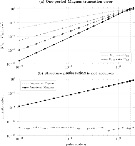
One-period benchmark for $e^Ye^X$. The upper panel shows the four cumulative Magnus errors. The lower panel contrasts the binary64 unitarity floor of the exponentiated fourth-degree truncation with the growing defect of the degree-two Dyson polynomial. The vertical line is the sufficient-bound threshold $\eta=\pi/1.8$; it is not an accuracy contour.

Unitarity Is Not Accuracy

All four Magnus approximations have maximum one-period unitarity defect $1.12\times10^{-15}$ over the full sweep $0.01\le\eta\le2$. Their operator errors range from below $10^{-11}$ to order unity. Exact structural preservation says that a computation stays on the unitary group; it does not say that it reaches the correct point on that group.

The Dyson control makes the distinction visible.

$\eta$	Fourth-degree Magnus error	Magnus unitarity defect	Dyson error	Dyson unitarity defect
0.05	$1.61\times10^{-8}$	$9.20\times10^{-16}$	$1.12\times10^{-4}$	$1.40\times10^{-5}$
0.16	$5.45\times10^{-6}$	$2.81\times10^{-16}$	$3.67\times10^{-3}$	$1.47\times10^{-3}$
0.32	$1.79\times10^{-4}$	$4.26\times10^{-16}$	$2.92\times10^{-2}$	$2.35\times10^{-2}$
0.64	$6.24\times10^{-3}$	$5.69\times10^{-17}$	$2.30\times10^{-1}$	$3.76\times10^{-1}$
1.50	$5.19\times10^{-1}$	$4.67\times10^{-16}$	$2.64$	$11.34$

The lesson is asymmetric. A large unitarity defect certifies a structural failure, but a tiny defect does not certify dynamical accuracy.

Pulse Order and Commutators

Reversing the pulses changes the exact propagator from $e^Ye^X$ to $e^Xe^Y$. The leading average $X+Y$ is unchanged, while

$$\frac12[Y,X] \longrightarrow \frac12[X,Y] = -\frac12[Y,X].$$

The program verifies the sign reversal with Frobenius residual zero in binary64 for every sampled $\eta$. The exact forward and reverse propagators differ by $0.02876$ at $\eta=0.16$ and $0.41377$ at $\eta=0.64$. Thus pulse order is not a cosmetic convention once the generators fail to commute.

As an independent control, replacing the second axis by $\sigma_x$ gives $[Y,X]=0$. At $\eta=0.9$, the first Magnus exponential then agrees with the exact product to $2.22\times10^{-16}$, and the computed commutator norm is exactly zero.

These checks probe algebra rather than convergence. They can catch a mistaken matrix multiplication order even when a log-log slope happens to look plausible.

The Sufficient Convergence Bound

For a bounded matrix generator $A(t)$, a standard sufficient condition for convergence of the Magnus series on an interval is

$$\int_0^T \|A(t)\|_2\,dt \lt \pi.$$

Here the two pulse areas give

$$\int_0^1 \|A(t)\|_2\,dt = \eta+0.8\eta = 1.8\eta,$$

so the condition holds for

$$\eta \lt \frac{\pi}{1.8} \approx 1.74533.$$

Three distinctions are essential.

1. The condition is sufficient, not necessary. Its failure at $\eta=2$ does not by itself prove divergence.
2. It concerns convergence of the infinite Magnus series, not the accuracy of a fixed low-degree truncation.
3. It does not imply that successive low-degree propagators improve monotonically.

At $\eta=1.5$, where $1.8\eta=2.7<\pi$, the third-degree operator error is $0.3775$ and the fourth-degree error is $0.5194$. The infinite series may converge while a particular early partial sum overshoots. A practical calculation still needs a truncation-error study.

Stroboscopic Accumulation

The repeated-period test fixes $\eta=0.16$ and computes

$$U_{\mathrm{ex}}^n, \qquad \left(U_M^{[r]}\right)^n, \qquad 1\le n\le200.$$

Every matrix power remains unitary to floating-point precision. Nevertheless, a small error in the effective rotation angle or axis accumulates coherently.

Periods $n$	Exact $P(n)$	Third-degree operator error	Fourth-degree operator error	Fourth-degree probability error
1	0.061277	$6.96\times10^{-5}$	$5.45\times10^{-6}$	$2.15\times10^{-6}$
10	0.188288	$1.23\times10^{-4}$	$5.27\times10^{-5}$	$3.88\times10^{-5}$
25	0.117252	$1.03\times10^{-4}$	$1.32\times10^{-4}$	$7.85\times10^{-5}$
50	0.406890	$1.93\times10^{-4}$	$2.63\times10^{-4}$	$2.31\times10^{-4}$
100	0.879507	$3.01\times10^{-4}$	$5.26\times10^{-4}$	$7.17\times10^{-5}$
200	0.022949	$2.93\times10^{-4}$	$1.05\times10^{-3}$	$2.95\times10^{-4}$

The fourth-degree approximation wins clearly at one period, but its operator error exceeds the third-degree error by $n=25$. Different truncations perturb the exact rotation angle and axis in different directions, so finite-time cancellation can reverse their ranking. The errors also oscillate rather than growing monotonically because all propagators remain on the compact group $SU(2)$.

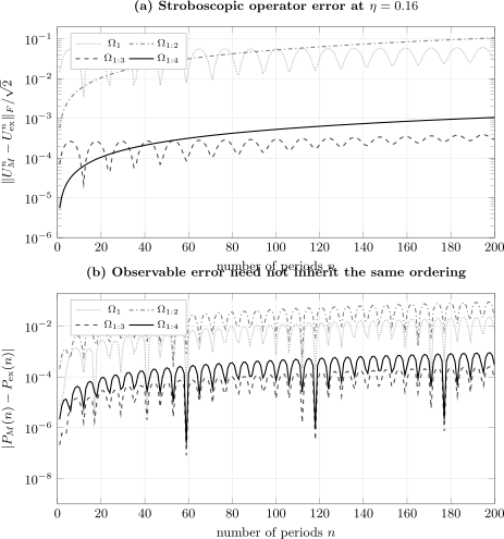
Repeated-period errors at $\eta=0.16$. The upper panel uses a state-independent operator norm; the lower panel uses the single transition probability $P(n)=|\langle1|U^n|0\rangle|^2$. Oscillations and crossings show why one-period order, long-time operator error, and one chosen observable are distinct diagnostics.

Effective-Hamiltonian Branches

Writing the exact one-period unitary as

$$U_{\mathrm{ex}} = e^{-iH_FT}$$

does not determine a unique Hermitian $H_F$. If

$$U_{\mathrm{ex}}|\phi_a\rangle = e^{-i\epsilon_aT}|\phi_a\rangle,$$

then every replacement

$$\epsilon_a \longrightarrow \epsilon_a + \frac{2\pi k_a}{T}, \qquad k_a\in\mathbb Z,$$

reconstructs the same one-period unitary.

At $\eta=0.64$ and $T=1$, the principal generator has quasienergies $\epsilon_-= -1.0560023774$ and $\epsilon_+=1.0560023774$. Representative branches are

Lower shift	Upper shift	$\epsilon_-$	$\epsilon_+$	Reconstruction error
0	0	$-1.056002$	$1.056002$	$2.67\times10^{-16}$
0	1	$-1.056002$	$7.339188$	$7.36\times10^{-16}$
1	1	$5.227183$	$7.339188$	$1.76\times10^{-15}$

The full nine-branch table, with independent shifts $k_-,k_+\in\{-1,0,1\}$, has maximum reconstruction error $2.12\times10^{-15}$. A matrix logarithm routine returning the principal branch has made a convention choice, not discovered a unique physical spectrum.

The Magnus series expanded continuously from $\eta=0$ selects the logarithm branch analytic near the identity. Tracking a physically continuous branch through a quasienergy-zone boundary is a separate spectral problem; the Floquet Quasienergy Notebook treats that task directly.

Validation Ledger

The retained program aborts if any required check fails.

Check	Result	Interpretation
fitted Magnus powers	1.9994, 3.0016, 3.9996, 5.0009	correct first omitted degrees
largest one-period Magnus unitarity defect	$1.12\times10^{-15}$	exponentiation preserves structure
largest exact-unitary defect	$4.44\times10^{-16}$	analytic product is numerically stable
largest exact determinant defect	$4.44\times10^{-16}$	propagators remain in $SU(2)$
largest second-term reversal residual	$0$	pulse order gives the correct sign
commuting-control error	$2.22\times10^{-16}$	first term becomes exact when it should
Dyson defect at $\eta=0.64$	$0.37583$	nonunitary control is visibly diagnostic
largest branch reconstruction error	$2.12\times10^{-15}$	shifted logarithms reproduce the same $U_F$
largest 200-period Magnus unitarity defect	$1.57\times10^{-13}$	repeated products show only roundoff-level drift

These checks are deliberately heterogeneous. Weak-drive slopes test truncation degree; pulse reversal tests algebra; commuting pulses test an exact limit; unitarity tests group structure; branches test logarithm conventions; stroboscopic powers test accumulated dynamical error.

Reproduce the Calculation

Run the downloaded program from the folder where you saved it:

python magnus-expansion-error.py --output-dir results

The deterministic program uses NumPy only. Adding --plot generates optional Matplotlib quick-look plots, but the published SVG figures are rendered from the retained CSV tables with PGFPlots and TikZ.

Retained artifacts

• Python program
• One-period error sweep
• Stroboscopic sweep
• Effective-Hamiltonian branch table
• One-period figure source
• Stroboscopic figure source

Reproducibility metadata

Item	Retained setting
Python	3.12.13 in the recorded production run
NumPy	2.3.5
arithmetic	IEEE 754 binary64 complex matrices
matrix size	$2\times2$
sweep	18 fixed $\eta$ values from $0.010$ to $2.000$
slope fit	ordinary least squares in log space for $\eta\le0.075$
stroboscopic run	$\eta=0.16$, $n=1,\ldots,200$
branch run	$\eta=0.64$, shifts $k_-,k_+\in\{-1,0,1\}$
randomness	none
production runtime	0.034 s on the recorded machine
program license	MIT, identified by an SPDX header

The exact propagator, Pauli exponentials, and truncated generators are evaluated directly. No adaptive tolerance, hidden optimizer, numerical time step, or random seed influences the quoted values.

Known Failure Modes

• Wrong product order: if pulse $A$ acts first, its propagator belongs on the right of $U_B U_A$.
• Term versus truncation confusion: $\Omega_4$ alone is not the generator through fourth degree.
• Unitarity as certification: exponentiating any anti-Hermitian approximation gives a unitary matrix, including an inaccurate one.
• Bound overinterpretation: $\int\|A\|dt<\pi$ is a sufficient series-convergence condition, not a fixed-order error estimate.
• Branch-blind generator comparison: two effective Hamiltonians can differ by spectral shifts of $2\pi/T$ and generate the same stroboscopic unitary.
• One observable only: a transition probability can hide operator error through projection or cancellation.
• One period only: a tiny local error may accumulate coherently over many cycles.
• Near-cut ambiguity: the principal matrix logarithm changes discontinuously when an eigenphase crosses its branch cut.
• Floating-point floor: unitarity defects near $10^{-15}$ measure binary64 roundoff, not a physical approximation error.

Further Investigations

1. Replace the two-step cycle by a time-symmetric $A/2$–$B$–$A/2$ sequence and verify the cancellation of the appropriate even Magnus contributions.
2. Smooth the pulse discontinuity while preserving the integrated areas, then compare numerical time integration with the exact step-drive benchmark.
3. Fit effective rotation-axis and rotation-angle errors separately to identify which component controls the long-time crossings.
4. Track a continuous quasienergy branch as $\eta$ passes a principal-logarithm cut.
5. Repeat the calculation in higher precision to separate matrix-exponential roundoff from asymptotic truncation error below $10^{-14}$.
6. Extend the drive to a larger Hilbert space, where spectral crowding and operator-norm bounds become substantially more restrictive.

Exercises

1. Compute the leading commutator

Evaluate $\Omega_2=\tfrac12[Y,X]$ for the two pulse generators and identify its Pauli direction.

Solution

Using $[\sigma_i,\sigma_j]=2i\epsilon_{ijk}\sigma_k$,

$$\begin{aligned} [Y,X] &= (-i)^2 \frac{0.8\eta^2}{\sqrt2} [\sigma_x+\sigma_z,\sigma_x] \\ &= -\frac{0.8\eta^2}{\sqrt2} [\sigma_z,\sigma_x] \\ &= -i\frac{1.6\eta^2}{\sqrt2} \sigma_y. \end{aligned}$$

Therefore

$$\Omega_2 = -i\frac{0.8\eta^2}{\sqrt2} \sigma_y.$$

The leading time-ordering correction points along $y$, perpendicular to the plane spanned by the two pulse axes. Reversing the pulses changes its sign.

2. Prove finite-truncation unitarity

Show that $U_M^{[r]}$ is unitary whenever the Hamiltonian is Hermitian, even before the Magnus series has converged to the exact propagator.

Solution

For Hermitian $H(t)$, the differential generator $A(t)=-iH(t)/\hbar$ is anti-Hermitian. Integrals, real linear combinations, and commutators of anti-Hermitian matrices are anti-Hermitian in the combinations appearing in each Magnus term. Hence

$$\left( \sum_{j=1}^{r}\Omega_j \right)^\dagger = - \sum_{j=1}^{r}\Omega_j.$$

Writing the sum as $K_r$ gives

$$\begin{aligned} \left(e^{K_r}\right)^\dagger e^{K_r} &= e^{K_r^\dagger}e^{K_r} \\ &= e^{-K_r}e^{K_r} =I. \end{aligned}$$

No claim about $e^{K_r}=U_{\mathrm{ex}}$ was used. Structure preservation and approximation accuracy are logically separate.

3. Infer an observed order

Suppose the fourth-degree errors at $\eta=0.16$ and $\eta=0.32$ are $5.4470\times10^{-6}$ and $1.7893\times10^{-4}$. Estimate the two-point convergence power.

Solution

For $\epsilon(\eta)\propto\eta^p$,

$$p = \frac{ \log \left[ \epsilon(0.32)/\epsilon(0.16) \right] }{ \log(0.32/0.16) }.$$

Substitution gives

$$p \approx \frac{\log(32.85)}{\log2} \approx 5.04.$$

This is consistent with the expected $O(\eta^5)$ error. The production fit uses six points with $\eta\le0.075$ to reduce finite-coupling contamination.

4. Interpret the norm threshold

The integrated norm is $1.8\eta$. Classify $\eta=1.5$ and $\eta=2.0$ under the sufficient convergence condition, and state what can be concluded about the fourth-degree approximation.

Solution

At $\eta=1.5$,

$$1.8\eta=2.7<\pi,$$

so the standard sufficient condition guarantees convergence of the full Magnus series. It does not guarantee that fourth degree is accurate or better than third degree; the measured errors show that it is worse here.

At $\eta=2.0$,

$$1.8\eta=3.6>\pi.$$

The sufficient condition no longer applies. One cannot infer divergence from that failure, and one still must measure the truncation error directly.

5. Construct an equivalent Floquet branch

At $T=1$, shift only the upper principal quasienergy $1.0560023774$ by one Floquet zone. Find the new quasienergy and show why the one-period eigenvalue is unchanged.

Solution

One zone has width $2\pi/T=2\pi$, so

$$\begin{aligned} \epsilon_+' &= 1.0560023774+2\pi \\ &\approx 7.3391876846. \end{aligned}$$

Its eigenvalue is

$$\begin{aligned} e^{-i\epsilon_+'T} &= e^{-i(\epsilon_++2\pi)T} \\ &= e^{-i\epsilon_+T}e^{-i2\pi} \\ &= e^{-i\epsilon_+T}. \end{aligned}$$

The effective Hamiltonian changes, but the sampled one-period propagator does not.

6. Bound repeated-period operator error

For unitary matrices $U$ and $V$, derive the bound $\|U^n-V^n\|\le n\|U-V\|$ for any unitarily invariant norm. Why can the measured error be much smaller or oscillatory?

Solution

Use the telescoping identity

$$U^n-V^n = \sum_{j=0}^{n-1} U^{n-1-j}(U-V)V^j.$$

Unitary invariance and the triangle inequality give

$$\begin{aligned} \|U^n-V^n\| &\le \sum_{j=0}^{n-1} \left\| U^{n-1-j}(U-V)V^j \right\| \\ &= n\|U-V\|. \end{aligned}$$

This is a worst-case upper bound. The matrix terms in the sum can point in different operator directions and partially cancel. On $SU(2)$, both evolutions are bounded rotations, so their separation can grow, shrink, and recur rather than increasing monotonically.

Cross-Links

• Computational Notebooks defines the validation and reproducibility contract used here.
• Magnus Expansion derives the general nested-commutator series.
• Floquet–Magnus Expansion explains the one-period effective generator and its drive-phase dependence.
• Average Hamiltonian Theory develops pulse-cycle applications in a toggling frame.
• Dyson Expansion for Transition Amplitudes provides the polynomial-series comparison.
• Floquet Operators gives the canonical quasienergy and micromotion framework.
• Floquet Quasienergy Notebook follows branch continuity through avoided crossings and zone edges.
• Convergence Tests develops reusable observed-order and refinement diagnostics.

References

1. W. Magnus, “On the exponential solution of differential equations for a linear operator,” Communications on Pure and Applied Mathematics 7, 649–673 (1954), doi:10.1002/cpa.3160070404.
2. S. Blanes, F. Casas, J. A. Oteo, and J. Ros, “The Magnus expansion and some of its applications,” Physics Reports 470, 151–238 (2009), doi:10.1016/j.physrep.2008.11.001.
3. P. C. Moan and J. Niesen, “Convergence of the Magnus series,” Foundations of Computational Mathematics 8, 291–301 (2008), doi:10.1007/s10208-007-9010-0.
4. F. Casas, “Sufficient conditions for the convergence of the Magnus expansion,” Journal of Physics A: Mathematical and Theoretical 40, 15001–15017 (2007), doi:10.1088/1751-8113/40/50/006.
5. N. J. Higham, Functions of Matrices: Theory and Computation, SIAM (2008), doi:10.1137/1.9780898717778.
6. E. Hairer, C. Lubich, and G. Wanner, Geometric Numerical Integration, 2nd ed., Springer (2006), doi:10.1007/3-540-30666-8.
7. M. Bukov, L. D’Alessio, and A. Polkovnikov, “Universal high-frequency behavior of periodically driven systems: from dynamical stabilization to Floquet engineering,” Advances in Physics 64, 139–226 (2015), doi:10.1080/00018732.2015.1055918.