Average Hamiltonian Theory

Average Hamiltonian theory replaces a rapid, usually periodic control cycle by the effective Hamiltonian that generates its stroboscopic evolution. It began as the language of coherent averaging in nuclear magnetic resonance (NMR), where pulse sequences can suppress dipolar broadening while retaining selected spin interactions. The same construction now organizes composite pulses, Hamiltonian engineering, dynamical decoupling, and digital or analog quantum simulation.

“Average” here does not mean an expectation value in a state. It means an operator obtained from the logarithm of a one-cycle propagator. The ordinary time average is only its leading term:

$$\begin{aligned} U(T_c) &= \exp\left( -\frac{i}{\hbar}\overline H T_c \right), \\ \overline H &= \overline H^{(0)} +\overline H^{(1)} +\cdots. \end{aligned}$$

This page owns the control-cycle formulation: toggling frames, piecewise pulse sequences, zeroth-order selection rules, commutator corrections, cycle symmetries, and finite-pulse diagnostics. Magnus Expansion owns the general exponential series and its derivation. Dynamical Decoupling owns noise spectra, filter functions, and named protection sequences. Links to Quantum Control places all three in the wider pulse- and gate-design workflow.

Periodic Control Problem

Separate the Hamiltonian into an internal or drift part and an applied control:

$$H(t)=H_{\mathrm{int}}(t)+H_c(t).$$

Let the control propagator satisfy

$$i\hbar\dot U_c(t) = H_c(t)U_c(t), \qquad U_c(0)=I.$$

Factor the full propagator as

$$U(t)=U_c(t)\widetilde U(t).$$

Substitution into the Schrödinger equation gives the exact toggling-frame evolution

$$i\hbar\frac{d\widetilde U}{dt} = \widetilde H(t)\widetilde U(t),$$

with

$$\widetilde H(t) = U_c^\dagger(t) H_{\mathrm{int}}(t) U_c(t).$$

The strong control has disappeared from the generator because it is represented exactly by $U_c(t)$. Its effect is to rotate, switch, or otherwise modulate the internal Hamiltonian.

Cyclic control

Choose a cycle duration $T_c$ for which

$$U_c(T_c)=e^{i\phi_c}I.$$

The irrelevant scalar phase may be set to one. If the control waveform and internal Hamiltonian repeat, then $\widetilde H(t+T_c)=\widetilde H(t)$. Define the exact cycle Hamiltonian by

$$\begin{aligned} \widetilde U(T_c) &= \mathcal T \exp\left[ -\frac{i}{\hbar} \int_0^{T_c}\widetilde H(t)\,dt \right], \\ &= \exp\left( -\frac{i}{\hbar}\overline H T_c \right). \end{aligned}$$

At integer numbers of cycles,

$$\widetilde U(nT_c) = \left[\widetilde U(T_c)\right]^n = \exp\left( -\frac{i}{\hbar}\overline H\,nT_c \right).$$

The exact equality requires a consistent branch of the logarithm. Different branches shift quasienergies by integer multiples of $2\pi\hbar/T_c$. If $U_c(T_c)$ does not close, its net rotation must be included in the one-cycle propagator rather than silently discarded.

Average Hamiltonian theory is therefore naturally stroboscopic. Motion within a cycle is micromotion and generally cannot be reconstructed from $\overline H$ alone.

Piecewise Pulse Sequences

Ideal hard-pulse models divide the cycle into free intervals separated by instantaneous control unitaries. Let $P_j$ be pulse $j$, and define the cumulative control after that pulse by

$$G_j=P_jP_{j-1}\cdots P_1, \qquad G_0=I.$$

During a free interval of duration $\tau_j$ after $j$ pulses, a time-independent internal Hamiltonian becomes

$$\widetilde H_j = G_j^\dagger H_{\mathrm{int}}G_j.$$

Cycle closure requires $G_m=e^{i\phi_c}I$ after the final pulse, and

$$T_c=\sum_{j=0}^{m-1}\tau_j$$

in the zero-width pulse idealization.

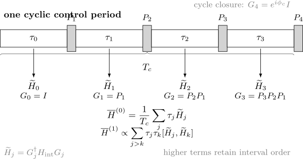
Control pulses change the cumulative frame $G_j$, so the same internal Hamiltonian appears as $\widetilde H_j=G_j^\dagger H_{\mathrm{int}}G_j$ in interval $j$. The weighted sum gives $\overline H^{(0)}$; ordered commutators of different intervals give higher terms.

The toggling frame converts pulse design into Hamiltonian design. Instead of tracking a long product of pulse and free-evolution operators directly, one asks which rotated Hamiltonians appear, for how long, and in what order.

Finite pulses are not instantaneous boundaries. During a pulse of duration $\tau_p$, the internal Hamiltonian and control act simultaneously, so that interval must be included in $\widetilde H(t)$. The hard-pulse approximation requires at least

$$\frac{\tau_p\lVert H_{\mathrm{int}}\rVert}{\hbar}\ll 1$$

on the relevant subspace, together with adequate control-amplitude, detuning, leakage, and bandwidth checks.

Notation and experimental conventions for Ramsey, echo, CPMG, XY-family, and composite-pulse protocols are catalogued in Pulse Sequences.

Zeroth-Order Average Hamiltonian

The leading term is the cycle average of the toggling-frame Hamiltonian:

$$\overline H^{(0)} = \frac{1}{T_c} \int_0^{T_c}\widetilde H(t)\,dt.$$

For ideal piecewise-constant intervals,

$$\overline H^{(0)} = \sum_{j=0}^{m-1} \frac{\tau_j}{T_c}\widetilde H_j.$$

This is an operator-valued weighted average. It can:

• cancel an unwanted term by rotating it through signs or orientations whose weighted sum vanishes;
• retain a desired term that is invariant under every control operation;
• rescale an interaction by changing interval weights;
• transform an anisotropic coupling into one with a chosen symmetry;
• select one component of a larger operator decomposition.

The control cannot distinguish “desired” and “undesired” by intention. Any term transforms according to its operator structure. A sequence that removes dephasing may also remove a wanted signal or gate Hamiltonian unless that term lies in the retained symmetry sector.

Echo as exact commuting cancellation

For static qubit detuning,

$$H_{\mathrm{int}} = \frac{\hbar\delta}{2}Z,$$

an ideal $X$ pulse at half a cycle gives

$$\widetilde H(t) = \begin{cases} +\hbar\delta Z/2, &0\lt t\lt T_c/2, \\ -\hbar\delta Z/2, &T_c/2\lt t\lt T_c. \end{cases}$$

The zeroth-order average vanishes. Because the two interval Hamiltonians are proportional to $Z$, all their commutators vanish as well. In this ideal static model, cancellation is exact, not merely a lowest-order result. Bath evolution, time-dependent noise, transverse couplings, and pulse imperfections remove that special exactness.

Higher-Order Corrections

Noncommuting interval Hamiltonians remember their order. Applying the Magnus series to one toggling-frame cycle gives

$$\overline H = \overline H^{(0)} +\overline H^{(1)} +\overline H^{(2)} +\cdots.$$

Average-Hamiltonian indexing starts the time average at order zero. The first correction is

$$\begin{aligned} \overline H^{(1)} ={}& -\frac{i}{2\hbar T_c} \int_0^{T_c}dt_1 \int_0^{t_1}dt_2 \\ &\quad\times \left[ \widetilde H(t_1), \widetilde H(t_2) \right]. \end{aligned}$$

The second correction is

$$\begin{aligned} \overline H^{(2)} ={}& -\frac{1}{6\hbar^2T_c} \int_0^{T_c}dt_1 \int_0^{t_1}dt_2 \int_0^{t_2}dt_3 \\ &\quad\times \Big( [\widetilde H_1,[\widetilde H_2,\widetilde H_3]] \\ &\qquad+ [\widetilde H_3,[\widetilde H_2,\widetilde H_1]] \Big), \end{aligned}$$

where $\widetilde H_j=\widetilde H(t_j)$ only within this displayed formula.

For piecewise-constant free intervals, the first correction simplifies to

$$\overline H^{(1)} = -\frac{i}{2\hbar T_c} \sum_{j>k} \tau_j\tau_k [\widetilde H_j,\widetilde H_k].$$

There is no contribution from two times in the same interval because $[\widetilde H_j,\widetilde H_j]=0$. Reversing the interval order changes the sign of each pairwise commutator while leaving $\overline H^{(0)}$ unchanged. Two pulse cycles can therefore have the same time fractions and different effective Hamiltonians.

Expansion parameter

If $\lVert\widetilde H(t)\rVert$ is characterized by an energy scale $h$, then the natural cycle parameter is

$$\lambda=\frac{hT_c}{\hbar}.$$

Dimensionally,

$$\overline H^{(n)} \sim h\lambda^n.$$

Fast cycling means $\lambda\ll1$ on the retained subspace. A standard sufficient Magnus convergence condition is

$$\frac{1}{\hbar} \int_0^{T_c} \lVert\widetilde H(t)\rVert\,dt \lt \pi.$$

It is sufficient rather than necessary, and it can be unhelpful for unbounded or extensive many-body Hamiltonians. In those settings, locality, energy density, resonances, and prethermal time windows can matter more than the global norm. A truncated average Hamiltonian should be validated against the exact one-cycle propagator or a converged numerical calculation whenever feasible.

Accumulation over many cycles

An exact $\overline H$ reproduces all integer-cycle evolution. A truncation leaves a one-cycle error that can accumulate with the number of repetitions. If the per-cycle propagator error is $\epsilon_c$, a conservative short-time estimate is often proportional to $n\epsilon_c$ after $n$ cycles, until interference, instability, or saturation changes the behavior. Small $T_c$ alone does not certify arbitrarily long evolution.

Sequence Symmetry

Symmetry can remove whole classes of commutator corrections without evaluating them term by term.

If the complete toggling-frame cycle is symmetric about its midpoint,

$$\widetilde H(t) = \widetilde H(T_c-t),$$

then the odd average-Hamiltonian orders vanish:

$$\overline H^{(1)} = \overline H^{(3)} = \overline H^{(5)} = \cdots = 0.$$

In Magnus notation these correspond to the even Magnus exponents $\Omega_2,\Omega_4,\ldots$. The distinction is purely indexing: $\overline H^{(0)}$ comes from $\Omega_1$.

A practical way to create this symmetry is a palindromic cycle: traverse a set of toggling-frame intervals and then retrace them in reverse order with matching durations. The statement applies to the full Hamiltonian during the full cycle. Treating pulses as finite can break a symmetry that appears exact in a delta-pulse diagram unless the pulse shapes are also arranged symmetrically.

Time antisymmetry and phase-cycling symmetries can impose other selection rules, but they must be derived for the actual toggling-frame Hamiltonian rather than inferred from a visually balanced pulse diagram.

Group Averaging and the Commutant

Suppose the control visits every element of a finite unitary group $\mathcal G$ for equal durations. Zeroth-order averaging defines

$$\Pi_{\mathcal G}(H) = \frac{1}{\lvert\mathcal G\rvert} \sum_{g\in\mathcal G} g^\dagger Hg.$$

For any $h\in\mathcal G$,

$$h^\dagger \Pi_{\mathcal G}(H) h = \Pi_{\mathcal G}(H).$$

Thus the group average lies in the commutant of the control representation: it retains exactly the operator components invariant under conjugation by the group. With the Hilbert–Schmidt inner product in finite dimensions, $\Pi_{\mathcal G}$ is the projector onto that invariant operator subspace.

Single-qubit Pauli average

Write a general qubit–bath interaction as

$$\begin{aligned} H ={}& I\otimes B_0 +X\otimes B_x \\ &+ Y\otimes B_y +Z\otimes B_z. \end{aligned}$$

Average over

$$\mathcal G=\{I,X,Y,Z\},$$

with global phases ignored. Conjugation by the Pauli operators changes the signs of the nonidentity Pauli components. Their four contributions cancel, leaving

$$\Pi_{\mathcal G}(H) = I\otimes B_0.$$

This is the algebraic core of universal first-order qubit decoupling. It does not by itself guarantee practical coherence protection: higher commutators, finite pulses, bath evolution, control errors, and noise above the cycle rate remain.

Selective Averaging in NMR

For two spins $I$ and $S$, a secular dipolar coupling aligned with the laboratory $z$ axis has the schematic form

$$H_{D,z} = d\left( 2I_zS_z -I_xS_x -I_yS_y \right).$$

Ideal rotations can permute the distinguished axis, producing

$$\begin{aligned} H_{D,x} &= d\left( 2I_xS_x-I_yS_y-I_zS_z \right), \\ H_{D,y} &= d\left( 2I_yS_y-I_zS_z-I_xS_x \right). \end{aligned}$$

The three orientations obey

$$H_{D,x}+H_{D,y}+H_{D,z}=0.$$

Equal time in these orientations therefore removes this ideal dipolar interaction from $\overline H^{(0)}$. This identity is an algebraic core of multiple-pulse dipolar averaging in solid-state NMR. It is not a complete specification of WAHUHA or any laboratory sequence: real designs must also track chemical shifts, scalar couplings, pulse phases, receiver timing, finite widths, and higher-order terms.

The broader NMR goal is selective averaging. One engineers a control cycle whose invariant operator sector contains useful chemical-shift or coupling information while strong broadening terms average away. Average Hamiltonian theory supplies both the leading selection rule and the corrections that limit spectral resolution.

Relation to Magnus and Floquet Methods

The same one-cycle propagator appears in several languages:

Language	Primary question	Characteristic emphasis
Magnus expansion	How is a time-ordered exponential written as one exponential?	General nested-commutator series and convergence
Average Hamiltonian theory	What stroboscopic interaction does a control cycle engineer?	Toggling frame, pulse intervals, symmetries, retained terms
Floquet–Magnus expansion	What high-frequency Floquet Hamiltonian and micromotion describe a periodic drive?	Quasienergy branches, drive-frequency expansion, Floquet gauge
Rotating-wave approximation	Which terms remain near resonance in a rotating frame?	Resonant selection and counter-rotating corrections

Average Hamiltonian theory is a Magnus expansion applied after a control-defined frame transformation and organized cycle by cycle. Its conventional order labels are shifted by one relative to the $\Omega_n$ labels:

$$\overline H^{(n-1)} = \frac{i\hbar}{T_c}\Omega_n(T_c).$$

The exact cycle Hamiltonian is also a Floquet Hamiltonian. Changing the cycle origin $t_0$ changes

$$U(t_0+T_c,t_0)$$

by a micromotion conjugation. Exact quasienergies are unchanged, but the matrix representation of the effective Hamiltonian and any finite-order truncation can depend on that choice. A reported average Hamiltonian should therefore state the frame, cycle origin, and logarithm branch.

Dynamical Decoupling Preview

Dynamical decoupling uses control cycles to suppress system–environment coupling. At zeroth order, group or sign averaging can remove selected error operators. Higher average-Hamiltonian terms diagnose coherent residual couplings generated by noncommuting toggling-frame pieces.

That operator calculation is only one view of decoupling. For classical or quantum noise with temporal structure, pulse timing determines a frequency-domain filter. A sequence with a vanishing static average can still transmit noise near its filter peaks, and no finite-bandwidth control removes arbitrary Markovian relaxation. The canonical treatment of spin echo, CPMG, Uhrig timing, filter functions, and sensing tradeoffs is Dynamical Decoupling.

The quantum-information deployment workflow owns scheduler-constrained placement, frame-aware ideal-action checks, protected-estimand and cost records, and held-out deployment decisions; this page retains toggling-frame and Magnus calculations.

Use average Hamiltonian theory when the cycle is rapid enough that coherent operator corrections are the natural diagnostic. Use filter-function or open-system methods when the noise spectrum, bath correlation time, dissipation, or measured coherence envelope is central. Many experiments require both.

Practical Workflow

1. Declare the laboratory Hamiltonian. Separate drift, desired interactions, errors, bath terms, and applied control without omitting terms merely because the sequence is intended to cancel them.
2. Choose the control frame. Compute $U_c(t)$ and include its time ordering if the control axes do not commute.
3. Check cycle closure. Record $U_c(T_c)$, the cycle origin, and any net phase or rotation.
4. Construct the toggling Hamiltonian. Include free intervals and finite pulse intervals at the level of accuracy required.
5. Compute $\overline H^{(0)}$. Identify which operator components vanish, survive, or are rescaled.
6. Exploit exact symmetries. Use group, time, or phase symmetry only after verifying it for the full toggling-frame cycle.
7. Estimate higher terms. Evaluate the leading nonzero commutators and the parameter $T_c\lVert\widetilde H\rVert/\hbar$.
8. Benchmark the cycle propagator. Compare the truncated exponential with exact propagation for representative parameters.
9. Test repeated evolution. Validate the observables over the actual number of cycles, not only after one cycle.

Common Mistakes

• Calling $\overline H^{(0)}$ the exact average Hamiltonian when interval Hamiltonians do not commute.
• Averaging the laboratory-frame Hamiltonian without first transforming by the control propagator.
• Forgetting that the rightmost pulse acts first when constructing cumulative controls $G_j$.
• Treating a noncyclic control sequence as though its net pulse rotation were the identity.
• Ignoring the logarithm branch or cycle-origin dependence of an exact stroboscopic Hamiltonian.
• Assuming a small one-cycle correction stays small after arbitrarily many repetitions.
• Drawing instantaneous pulses while using hardware whose pulse duration is not negligible compared with internal dynamics.
• Using time symmetry to cancel odd orders while omitting asymmetric pulse shapes or delays.
• Canceling an unwanted operator without checking whether the same symmetry also cancels the desired signal.
• Equating zeroth-order dynamical decoupling with suppression of every noise frequency or dissipative channel.

References

• W. Magnus, “On the exponential solution of differential equations for a linear operator,” Communications on Pure and Applied Mathematics 7, 649–673 (1954), doi:10.1002/cpa.3160070404.
• J. S. Waugh, L. M. Huber, and U. Haeberlen, “Approach to high-resolution NMR in solids,” Physical Review Letters 20, 180–182 (1968), doi:10.1103/PhysRevLett.20.180.
• U. Haeberlen and J. S. Waugh, “Coherent averaging effects in magnetic resonance,” Physical Review 175, 453–467 (1968), doi:10.1103/PhysRev.175.453.
• U. Haeberlen, High Resolution NMR in Solids: Selective Averaging, Academic Press (1976).
• M. M. Maricq, “Application of average Hamiltonian theory to the NMR of solids,” Physical Review B 25, 6622–6632 (1982), doi:10.1103/PhysRevB.25.6622.
• S. Blanes, F. Casas, J. A. Oteo, and J. Ros, “The Magnus expansion and some of its applications,” Physics Reports 470, 151–238 (2009), doi:10.1016/j.physrep.2008.11.001.
• L. Viola, E. Knill, and S. Lloyd, “Dynamical decoupling of open quantum systems,” Physical Review Letters 82, 2417–2421 (1999), doi:10.1103/PhysRevLett.82.2417.
• L. Viola, S. Lloyd, and E. Knill, “Universal control of decoupled quantum systems,” Physical Review Letters 83, 4888–4891 (1999), doi:10.1103/PhysRevLett.83.4888.

Exercises

1. Derive the toggling-frame Hamiltonian

Let $U(t)=U_c(t)\widetilde U(t)$ with $i\hbar\dot U_c=H_cU_c$ and $H=H_{\mathrm{int}}+H_c$. Derive the equation obeyed by $\widetilde U(t)$.

Solution

Differentiate the factorization:

$$\dot U = \dot U_c\widetilde U +U_c\dot{\widetilde U}.$$

The full Schrödinger equation gives

$$i\hbar \left( \dot U_c\widetilde U +U_c\dot{\widetilde U} \right) = (H_{\mathrm{int}}+H_c) U_c\widetilde U.$$

Use $i\hbar\dot U_c=H_cU_c$ to cancel the control terms. Multiplying by $U_c^\dagger$ from the left gives

$$i\hbar\dot{\widetilde U} = U_c^\dagger H_{\mathrm{int}}U_c \widetilde U.$$

Therefore $\widetilde H=U_c^\dagger H_{\mathrm{int}}U_c$. The frame transformation is exact; approximation enters only when this toggling-frame evolution is truncated or ideal pulses are assumed.

2. Two noncommuting intervals

A cycle consists of $H_A$ for time $\tau_A$, followed by $H_B$ for time $\tau_B$. Find $\overline H^{(0)}$ and $\overline H^{(1)}$. What changes when the interval order is reversed?

Solution

With $T_c=\tau_A+\tau_B$,

$$\overline H^{(0)} = \frac{\tau_AH_A+\tau_BH_B}{T_c}.$$

In the first-order double integral, $t_1$ must lie in the later $B$ interval and $t_2$ in the earlier $A$ interval. Hence

$$\overline H^{(1)} = -\frac{i\tau_A\tau_B}{2\hbar T_c} [H_B,H_A].$$

Reversing the order leaves $\overline H^{(0)}$ unchanged but replaces $[H_B,H_A]$ by $[H_A,H_B]=-[H_B,H_A]$. The first correction changes sign.

3. Symmetrize a two-step cycle

Consider the palindromic cycle

$$H_A\ \text{for }\tau/2, \quad H_B\ \text{for }\tau, \quad H_A\ \text{for }\tau/2.$$

Show directly from the piecewise formula that $\overline H^{(1)}=0$.

Solution

Label the three intervals $0,1,2$ with

$$\begin{aligned} H_0&=H_A, & H_1&=H_B, \\ H_2&=H_A. \end{aligned}$$

and durations $\tau_0=\tau_2=\tau/2$, $\tau_1=\tau$. The pair $(1,0)$ contributes

$$\frac{\tau^2}{2}[H_B,H_A].$$

The pair $(2,1)$ contributes

$$\frac{\tau^2}{2}[H_A,H_B] = -\frac{\tau^2}{2}[H_B,H_A].$$

The pair $(2,0)$ vanishes because $[H_A,H_A]=0$. The sum is zero, so $\overline H^{(1)}=0$. This is the first nontrivial instance of the general time-symmetry rule.

4. Pauli-group decoupling

Verify explicitly that

$$\frac14 \sum_{g\in\{I,X,Y,Z\}} g^\dagger Xg=0,$$

and similarly for $Y$ and $Z$. What happens to a desired qubit Hamiltonian proportional to $Z$ under the same average?

Solution

Conjugating $X$ gives

$$\begin{array}{c|cccc} g & I & X & Y & Z\\ \hline g^\dagger Xg & X & X & -X & -X \end{array}$$

so the average vanishes. Cyclic permutations give the same cancellation for $Y$ and $Z$. Therefore every traceless single-qubit operator is removed, while the identity survives.

A desired Hamiltonian proportional to $Z$ is also removed. The group average recognizes operator symmetry, not experimental intention. To preserve a nontrivial gate while decoupling errors, one must modify the control construction, encode the system, or use dynamically corrected gates.

5. Dipolar orientation average

Using the three Hamiltonians $H_{D,x}$, $H_{D,y}$, and $H_{D,z}$ defined above, verify that equal weighting cancels the secular dipolar interaction at zeroth order. Does this prove exact cancellation?

Solution

Collect the coefficient of each Cartesian bilinear. For $I_xS_x$, the coefficients from the $x$, $y$, and $z$ orientations are $2,-1,-1$, whose sum is zero. The same pattern holds for $I_yS_y$ and $I_zS_z$. Therefore

$$\overline H_D^{(0)} = \frac13 \left( H_{D,x}+H_{D,y}+H_{D,z} \right) = 0.$$

This proves only zeroth-order cancellation. The differently oriented Hamiltonians generally do not commute, so higher average-Hamiltonian terms can survive. Finite pulses and other spin interactions add further corrections.

6. Finite-pulse audit

A nominal hard pulse has duration $\tau_p$, Rabi angular frequency $\Omega$, and acts while an internal scale $h$ remains present. State at least four dimensionless or operational checks needed before replacing the pulse by an instantaneous rotation.

Solution

Useful checks include:

1. $\tau_ph/\hbar\ll1$, so internal evolution during the pulse is small;
2. $\Omega\tau_p$ equals the intended rotation angle with the stated angular-frequency convention;
3. detuning satisfies $\lvert\Delta\rvert/\Omega\ll1$ for a resonant hard-pulse approximation;
4. amplitude and phase errors are small enough over all repeated pulses;
5. the control bandwidth does not excite leakage transitions;
6. rise time, ringing, and pulse overlap are negligible or modeled;
7. replacing finite pulses by exact pulse shapes does not materially change the one-cycle propagator;
8. accumulated error remains acceptable over the intended number of cycles.

Passing only the pulse-area check is insufficient because a correct net rotation can coexist with substantial internal evolution, leakage, or repeated coherent error.