Dynamical Decoupling

This page owns deployment and validation of dynamical decoupling for a declared idle or operation window; it does not own general filter-function or sequence theory. A deployment begins by naming the protected window, frame, subspace, ideal operation, and state, channel, or observable estimand, then asks whether a licensed sequence can be compiled, physically realized, and shown on paired held-out workloads to improve that estimand at acceptable total cost. Dynamical decoupling is open-loop physical suppression before measurement, not estimator postprocessing and not quantum-error-correction recovery. Because finite pulses, incompatible dynamics, irreducible noise, or resource cost can erase the modeled benefit, no decoupling is a legitimate and often informative outcome.

Required background. Noise, Channels, and Error Mitigation supplies the frozen task, system boundary, ideal operation, evidence, intervention, uncertainty, and total-cost record. Dynamical Decoupling supplies switching functions, spectral conventions, named sequence families, and the control-theory limits imported here rather than rederived.

Helpful background. Pulse Sequences supplies notation and sequence-family definitions; Average Hamiltonian Theory supplies toggling-frame and Magnus diagnostics; Pulse-Level Control supplies executable schedule representation; and Variance and Covariance supplies paired uncertainty propagation.

Dynamical Decoupling as a Compiled Control Intervention

Physical suppression precedes inference

Dynamical decoupling changes the physical evolution during the protected window. Open-loop control pulses repeatedly transform the system–environment interaction so that selected contributions cancel or acquire reduced spectral overlap under a stated model. Viola and Lloyd (1998) established this suppression idea for a two-state system, and Viola, Knill, and Lloyd (1999) formulated a broader group-averaging approach for open systems. Those theoretical constructions license candidate controls under assumptions; they do not themselves establish that a finite, calibrated schedule improves a contemporary workload.

The intervention therefore sits upstream of sampling. If a baseline channel is $\mathcal E_0$ and a realized controlled channel is $\mathcal E_{\mathrm{DD}}$ , subsequent measurements sample different physical channels. There is no estimator identity that converts one into the other after acquisition. By contrast, zero-noise extrapolation, probabilistic cancellation, measurement mitigation, and symmetry filtering change an inference rule or combine specially prepared records. Dynamical decoupling may be composed with those methods, but the downstream method must be recalibrated against $\mathcal E_{\mathrm{DD}}$ , not assumed to inherit evidence obtained for $\mathcal E_0$ .

Nor is repeated control a recovery protocol. No syndrome identifies which error occurred, no conditional inverse is applied, and no encoded correctability condition follows. A sequence can reduce a modeled coupling while leaving relaxation, within-subspace coherent error, leakage, and control faults. Calling the result “error corrected” would erase both the physical mechanism and the limits of the evidence.

This page owns deployment evidence

The canonical division of labor is operational. General sequence and filter theory remains with the control and open-systems pages; this page imports a frozen contract and decides whether a concrete control window passes compilation, physical, statistical, and cost tests.

Object	Canonical owner	Retained use on this page
Hahn, CPMG, XY, Uhrig, and composite-sequence definitions	Pulse Sequences and general Dynamical Decoupling	import a named and versioned sequence contract
switching functions, filter functions, spectral normalization, and sensing	general Dynamical Decoupling and Noise Spectra	apply one declared convention to a frozen deployment
toggling frames, Magnus terms, and group averaging	Average Hamiltonian Theory	check a supplied cancellation certificate and ideal net action
Markovianity, bath memory, dephasing, and relaxation models	Markovian and Non-Markovian Noise; Dephasing and Amplitude Damping	state the licensed model domain and irreducible floor
typed pulse IR, clock-grid alignment, resource occupancy, and frame propagation	Pulse-Level Control	determine whether the candidate schedule is realizable
pulse calibration, transfer functions, leakage, crosstalk, and heating	Control, Readout, and Calibration; Leakage and Crosstalk	charge measured nonidealities and epoch validity
selection, placement, protected estimand, paired validation, total cost, and stop decision	this page	provide the canonical QI deployment workflow
estimator mitigation, symmetry filtering, recovery, and fault tolerance	their specialist pages	define composition order and prevent category errors

This firewall prevents a convenient but invalid substitution: a named sequence is not deployment evidence. The accepted evidence bundle contains the original request, imported theory version, compiled schedule, pulse and frame realization, calibration epoch, matched comparator, all attempted records, uncertainty, cost, falsifiers, and final decision. Reporting Standards owns durable reporting infrastructure; the present page specifies the dynamical-decoupling fields that must enter it.

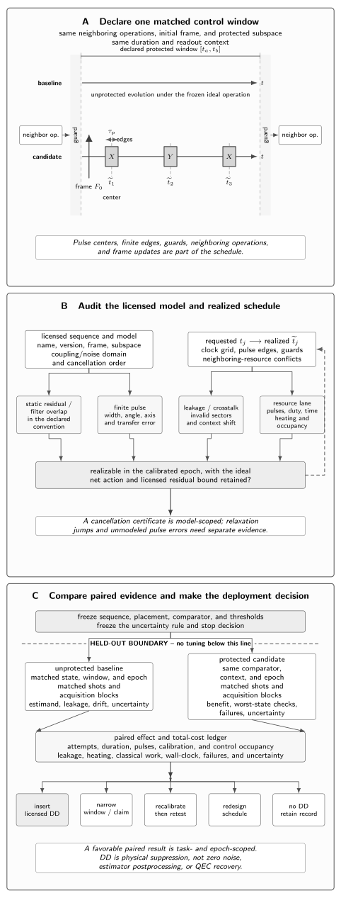
Dynamical-decoupling deployment audit from a declared control window through finite-pulse scheduling, model and cost checks, paired held-out validation, and an explicit deployment decision — A dynamical-decoupling deployment certificate connects a declared control window to a realizable finite-pulse schedule, licensed model, paired held-out evidence, full resource ledger, and explicit decision. General switching-function, filter, and named-sequence theory remains with the canonical control pages; the intervention is physical error suppression, not estimator postprocessing or QEC recovery.

Freeze the Protected Window and Estimand

The ideal operation depends on frame and subspace

A control window is not merely a duration. Record its start and end relative to neighboring operations, the physical qubits and couplers, the rotating or logical frame, the protected subspace $\mathcal H_{\mathrm p}$ , and all resources that must remain quiet or available. A nominal idle is the identity only in that declared frame and subspace. Static laboratory-frame precession, virtual frame advances, always-on interactions, and leakage-space phases may be intended evolution rather than noise.

Chronological order must be declared before any pulse product: physical operations act right-to-left. If $P_1$ occurs first and $P_N$ last, an idle deployment requires

P_N\cdots P_2P_1 = e^{i\phi}I_{\mathcal H_{\mathrm p}}.

The global phase $\phi$ is harmless only for the declared subspace and context. If relative phases arise between computational and leakage states, between spectator-conditioned blocks, or between branches later recombined, they are not one global phase. A protected gate is a stronger claim: the complete controlled evolution, including the desired dynamics between finite pulses and all declared frame changes, must approximate $U_{\mathrm{target}}$ on $\mathcal H_{\mathrm p}$ in a stated metric. An idle identity cannot certify that operation-level equality. Dynamically corrected gates are therefore a handoff unless the stronger product, subspace, frame, and error certificate is supplied.

The deployment certificate makes these dependencies reviewable.

Record	Required declaration	Executable or empirical check	Failure consequence
protected window	start, end, duration, boundary events, and eligible idle or operation class	compare compiled interval with the frozen request	reject placement or narrow the eligible window
frame and protected subspace	laboratory, rotating, logical, and virtual-frame conventions; projector onto $\mathcal H_{\mathrm p}$	propagate frames and test every basis state in the subspace	redesign; an apparent identity is not the declared identity
ideal target	$I_{\mathcal H_{\mathrm p}}$ for an idle or a specified $U_{\mathrm{target}}$ with metric and tolerance	multiply the complete ideal controlled product in chronological convention	reject an idle-only certificate for a protected gate
sequence name and version	family, source, parameterization, revision, and immutable identifier	resolve the identifier to one frozen sequence artifact	do not infer a schedule from a family label
axes, phases, and product convention	pulse axes, phases, angles, ordering, phase sign, and right-to-left action	reconstruct the ideal matrix or channel product	correct convention or reject
requested pulse centers	each $t_j$ relative to the window origin and whether it is a center	validate ordering, symmetry, and boundary request	return to sequence selection
realized centers and edges	snapped center and occupied interval $[t_j-\tau_j/2,t_j+\tau_j/2]$ for every pulse	recompute from emitted schedule and delivery trace	use realized, never requested, timing in predictions
pulse widths and shapes	$\tau_j$ , envelope, amplitude, carrier, phase, and integration convention	compare calibrated waveform and transfer-domain limits	recalibrate, replace, or reject pulses
boundary guards and clock grid	guard duration, tick size, rounding mode, and tie rule	snap all events and test edge clearance	shift, narrow, or reject the schedule
forbidden resource overlaps	drive, coupler, acquisition, reset, spectator, and concurrency exclusions	run resource-occupancy and neighboring-operation checks	reschedule or no decoupling
spectrum and model license	PSD convention, frequency band, stationarity, coupling, pulse approximation, and transfer domain	evaluate only inside licensed support and test diagnostic residuals	narrow the prediction or redesign the model
calibration epoch and transfer domain	calibration identifiers, timestamps, qubits, layouts, powers, temperatures, and validity limits	compare deployment context and drift sentinels with calibration	reacquire calibration before claiming transfer
estimand and matched comparator	state ensemble, channel metric, observable loss, workload, budget, and baseline schedule	compute paired protected-minus-baseline effect with common eligibility	report only the comparator actually tested
predeclared falsifier	minimum gain plus timing, leakage, worst-state, drift, and cost limits	evaluate every criterion including failures and dropped jobs	record the corresponding stop decision

State, channel, and observable comparators differ

A memory demonstration should state what information is protected. A favorable survival probability for $|0\rangle$ does not establish coherence; a favorable Ramsey contrast for one equatorial axis does not establish an unknown-state channel; and a favorable average over six cardinal states can conceal a failed worst state. A state-ensemble claim needs predeclared preparations, weights, measurement corrections, and a loss such as worst-state infidelity. A channel claim needs an accepted channel metric and sufficient characterization. A task-observable claim needs the exact circuit context, observable, estimator, and resource budget.

The comparator must match everything not intentionally changed. Use the same requested window class, device context, qubits, neighboring operations, state or workload distribution, acquisition eligibility, and analysis pipeline. If the DD schedule lengthens the physical interval, decide in advance whether the baseline receives an equal wait or whether wall-clock duration is itself part of the intervention. If extra calibration or failed jobs occur only for DD, retain them in its cost and unconditional outcome rather than conditioning them away.

The protected estimand may also contain useful signal evolution. A sign modulation that refocuses nuisance detuning can refocus the desired DC field or always-on interaction at the same time. For sensing, filter placement relative to a signal spectrum is often the objective, not an unwanted side effect; that protocol belongs with the general Dynamical Decoupling and sensing owners. Here the deployment record must state which desired term survives and test it. Noise suppression without target preservation is not benefit.

Import a Licensed Sequence Contract

A sequence name is not a specification

Historical names identify ideas, not executable schedules. Hahn (1950) established the single spin echo; Carr and Purcell (1954) introduced a repeated refocusing construction; Meiboom and Gill (1958) modified pulse phases to improve robustness for a particular magnetization setting. Uhrig (2007) derived nonuniform timings with high short-time cancellation order under specific coupling, cutoff, and ideal-pulse assumptions. Later XY and robust families add axes, phases, symmetry, concatenation, or composite pulses. None of the labels “echo,” “CPMG,” “XY,” or “UDD” determines pulse shape, width, phase convention, endpoint treatment, scheduler rounding, or hardware calibration.

Import an immutable sequence artifact that includes pulse axes and angles, requested center rule, cycle repetition, endpoint policy, frame convention, ideal product, and supported target class. Include the source and version. Souza, Álvarez, and Suter (2011) demonstrate why robust construction details matter: sequences designed to compensate pulse imperfections can behave differently from nominally equivalent phase patterns. Khodjasteh and Lidar (2005) analyze bounded-strength concatenated dynamical decoupling under a non-Markovian contract; “fault-tolerant” in that paper’s title must not be recast as fault-tolerant quantum computation.

The imported artifact is still a candidate. The compiler may be unable to honor its timing, resource, or waveform assumptions. If the artifact specifies instantaneous pulses while the hardware supplies forty-nanosecond waveforms, record that model gap and either license an approximation or use a finite-pulse model. Never silently turn pulse centers into leading edges, or requested times into realized times.

Noise, control, and desired-dynamics domains travel together

Every sequence claim has a domain. State the coupling operators to be modulated, the bath or stochastic model, its stationarity and spectral support, the control idealization, the initial-state or observable class, and the desired Hamiltonian that must remain. The Markovian and Non-Markovian Noise owner supplies the memory distinction; Dephasing and Amplitude Damping supplies the channel models. This page records which model is licensed for the deployment.

Cywiński et al. (2008) connect dephasing under pulse sequences to spectral filtering for specified classical or Gaussian environments. That analysis is useful when the measured or justified spectrum, pulse approximation, and coherence observable match. It is not permission to treat arbitrary non-Gaussian noise, strong coupling, leakage, relaxation, or correlated control faults as a scalar dephasing PSD. Likewise, an asymptotic cancellation order applies only where its expansion parameter is small and its cutoff assumptions hold.

Desired dynamics belong in the same contract because the toggling transformation acts on every Hamiltonian term. A sequence that averages $Z$ detuning can also average a wanted $Z$ rotation. Noncommuting target gates can be distorted differently in each interval. For a nominal idle, always-on two-qubit coupling or spectator-conditioned phase may still be desired, calibrated, or compensated. Freeze the allowed operation class and reject transfer to a different context until the ideal-action and empirical tests are repeated.

Compile Pulses into a Feasible Schedule

Pulse centers, edges, guards, and clock grid

Let the requested center of pulse $j$ be $t_j$ . A finite pulse of duration $\tau_j$ occupies

\left[t_j-\frac{\tau_j}{2},\, t_j+\frac{\tau_j}{2}\right].

Those endpoints, not the center alone, determine boundary and overlap safety. The schedule record must distinguish requested centers, snapped centers, leading and trailing edges, any rise or ring-down guard, and emitted start times. If the control system schedules leading edges, convert explicitly before comparing with a center-based sequence definition.

A timing grid needs both a spacing and a rule. Nearest-tick, floor, and ceiling snapping produce different modulation moments; ties require a deterministic convention. Snap the actual objects the backend snaps, then recompute all edges and free gaps. Preserving nominal symmetry by independently rounding centers is not guaranteed. If the sequence optimizer assumed continuous timing, the realized discrete schedule is a new candidate whose ideal product, static moment, and spectral score must be recalculated.

Boundary guards protect neighboring operations from waveform tails, resonator ring-down, phase transients, and resource acquisition. A center farther than the guard from an endpoint can still fail when half-width is included. Conversely, an endpoint pulse specified in ideal theory may be infeasible because its edge lies outside the declared window. Do not extend the window after seeing this failure unless the comparator and task contract are updated.

Resource conflicts and neighboring operations

The schedule uses physical resources beyond the driven qubit. Drives may share electronics; couplers may be reserved; acquisition, reset, flux excursions, or spectator pulses may forbid concurrency. Pulse-Level Control owns typed pulse representation, grid scheduling, frame propagation, lowering, and delivery provenance. The DD deployment supplies its requested window and consumes the emitted schedule plus a resource-occupancy certificate.

Check neighboring operations on both sides, not just overlaps among DD pulses. A guard can collide with measurement acquisition or a two-qubit gate even when every pulse lies inside the logical idle. Simultaneous DD on several qubits can violate aggregate power, crosstalk, or heating limits. Staggering sequences to pass those constraints changes their relative timing and may alter correlated-noise filtering. If the compiler serializes or drops pulses, the realized sequence must be renamed or rejected; it is not the requested contract.

Frame updates, net action, and scheduler rounding

Physical and virtual rotations must be propagated through the whole window. A virtual $Z$ update changes the phase of later equatorial pulses; a pulse phase specified in one rotating frame may implement a different axis after an intervening frame change. Reconstruct the emitted operation in one explicit convention, including compiler-inserted phase corrections. Test the net ideal action on every protected basis state and, when relevant, spectator-conditioned block.

For an idle, matrix equality up to one global phase is necessary. It is not sufficient: finite duration allows drift and coupling during the pulses, amplitude and detuning errors change rotation angles and axes, and schedule rounding changes free-evolution intervals. For a gate, compare the complete controlled product with $U_{\mathrm{target}}$ using a stated norm, infidelity, or diamond-distance bound appropriate to the claim. Average Hamiltonian Theory owns the toggling and Magnus derivations; this page checks the supplied certificate against the realized schedule.

Check the Ideal Controlled Evolution

Toggling signs give a static-noise audit

For ideal instantaneous sign-flipping pulses under pure dephasing, define

y(t)=(-1)^{n(t)}

between pulses, where $n(t)$ counts completed sign-flipping pulses. The accumulated phase from a static detuning $\xi_0$ is proportional to $\xi_0Y(0)$ , with

Y(0)=\int_0^T y(t)\,dt.

Thus $Y(0)=0$ is a direct quasistatic-cancellation check for that idealized schedule. It is sensitive to realized timing: shifts of pulse centers change signed interval lengths even when the ideal sequence was balanced.

Do not set $y(t)=\pm1$ during finite pulses unless a control approximation explicitly licenses it. While a pulse rotates the qubit, the toggling operator generally moves continuously and may have several components. One can omit pulse intervals only under a stated “dead-time” or strong-control approximation, or integrate a finite-pulse control matrix. The approximation and its error bound travel with the prediction.

A zero static moment is narrow evidence. It does not prove suppression at nonzero frequency, high-frequency robustness, Gaussianity, relaxation reversal, finite-pulse tolerance, or workload benefit. It can coexist with a large filter lobe, severe pulse error, or a sequence that cancels the desired signal. Report a nonzero residual even if it lies below a predeclared tolerance; passing a threshold does not make it exactly zero.

Filter overlap requires one spectral convention

For the imported two-sided angular-frequency convention,

\begin{aligned} Y(\omega,T) &= \int_0^T y(t)e^{i\omega t}\,dt,\\ \chi(T) &= \frac12 \int_{-\infty}^{\infty} \frac{d\omega}{2\pi}\, S_{\xi\xi}(\omega) \lvert Y(\omega,T)\rvert^2. \end{aligned}

Here $\xi$ is an angular-frequency fluctuation with units $\mathrm{s}^{-1}$ , $S_{\xi\xi}$ has units $\mathrm{s}^{-1}$ under the two-sided transform, and $Y$ has units $\mathrm{s}$ , so $\chi$ is dimensionless. More generally, if $\xi$ is assigned another physical unit, the coupling constant needed to form an angular frequency must appear explicitly. The $2\pi$ measure, two-sided symmetry, and definition of $Y$ cannot be borrowed from different conventions.

The coherence factor $e^{-\chi}$ follows only for the licensed dephasing model, commonly a stationary Gaussian classical process or a compatible weak-coupling treatment. A numerical quadrature additionally needs frequency nodes, weights, PSD units, interpolation, and support. The finite Audit 2 uses dimensionless weights as a declared toy discretization, not a noise-spectroscopy result. Control Limits and Noise owns broader control limits, while this page asks whether one frozen convention has been applied consistently.

Uhrig timing can produce a high-order short-time zero in a particular setting, whereas equidistant or robust sequences can perform better under different spectra and pulse constraints. Biercuk et al. (2009) experimentally studied optimized decoupling for a model trapped-ion memory, demonstrating the value of spectrum-aware design in that platform. It does not establish a universal sequence ranking or transfer unchanged to another cutoff, pulse width, or device.

Magnus cancellation and filtering order are different claims

A filter moment describes frequency response in a stated noise representation. A Magnus or average-Hamiltonian order describes which terms vanish in an expansion of toggling-frame evolution, subject to convergence and operator assumptions. An empirical order describes how a measured loss changes over a finite family of schedules. Similar powers of time can appear in all three, but they are not interchangeable certificates.

Paz-Silva and Viola (2014) develop generalized transfer functions precisely to organize control response beyond a single scalar dephasing filter. Their framework shows that cancellation order and filtering order can coincide only under additional structure; different fundamental filter functions and control paths can govern different noise terms. Therefore a claimed low-frequency zero must name the transfer function, while a Magnus claim must provide its operator expansion and domain.

The third claim—task improvement—requires data. Even a correct high-order theoretical certificate may lose to a lower-order sequence after finite widths, calibration error, bandwidth, leakage, or crosstalk are charged. Conversely, an empirical gain on one workload does not prove the theoretical order. Keep three separately labeled records: the moment or filter result, the average-Hamiltonian cancellation result, and the held-out loss difference.

Account for Finite Pulses and Control Error

Duration and duty cycle are physical costs

Finite pulses occupy time in which the ideal switching model is incomplete. Define the duty cycle as total occupied pulse time divided by the declared window, counting overlaps according to the relevant hardware resource. High duty can reduce free exposure to one noise source while increasing drive-induced dephasing, heating, leakage, or neighboring-qubit disturbance. If pulses extend the task duration, the added wall time can also increase relaxation.

The pulse count alone is not an adequate cost proxy. Two schedules with eight pulses can have different widths, amplitudes, shapes, bandwidths, energy, guards, and calibration burden. Audit 2 deliberately uses $(1-p)^8$ as an independent per-pulse toy proxy. That product is a predeclared score factor, not an identity for composing physical channels: real pulse faults may be coherent, correlated, state-dependent, and interleaved with environmental evolution.

Minimum spacing is likewise contextual. The hardware needs enough free gap for pulse edges, guards, and recovery of shared resources, while the model may need a shorter cycle than the noise correlation time. Ezzell et al. (2023) surveyed many dynamical-decoupling sequences on superconducting processors and found device- and context-dependent performance, directly cautioning against universal sequence or minimum-spacing rankings.

Amplitude, detuning, and axis errors accumulate

An intended $X_\pi$ pulse can carry rotation-angle error, detuning-induced axis tilt, quadrature imbalance, phase offset, and waveform distortion. Repeating the same imperfect axis can add coherently. Phase-alternating sequences may cancel selected systematic terms, but the cancellation license depends on input state, error stationarity, pulse symmetry, and cycle completion. It cannot be inferred from a family acronym.

Measure or bound pulse error in the same amplitude, duration, carrier, qubit, and neighboring-operation context as the deployment. A randomized average gate error alone may hide a coherent component that accumulates through the deterministic sequence. Conversely, a worst-case bound can be too conservative for a particular ensemble. Use the metric required by the protected estimand and propagate uncertainty into the predicted net benefit.

Calibration drift changes both the pulse and the baseline noise. Interleave drift sentinels, retain calibration timestamps, and predeclare when a changed frequency, amplitude, or transfer response invalidates the candidate. If retuning is triggered, classify the old held-out data as tuning evidence and acquire a new final comparison.

Leakage, crosstalk, heating, and calibration epoch limit transfer

Control can move population outside $\mathcal H_{\mathrm p}$ , disturb spectators, heat a device, or activate unwanted couplings. These outcomes are not captured by a computational-subspace identity or a dephasing filter. Leakage and Crosstalk owns enlarged-space and contextual error physics; the DD deployment must include measured leakage, spectator, and context falsifiers and charge every failed or unclassified record.

A sequence can improve a conditional computational-subspace score while increasing unconditional failure. Report both the protected estimand and leakage, loss, dropped-job, pulse-failure, and ambiguous-event rates using all eligible attempts. Do not remove failed DD jobs from the denominator unless the baseline uses the same predeclared eligibility rule. A “no encoding overhead” statement is irrelevant to pulse count, calibration shots, energy, resource occupancy, validation effort, or wall-clock cost.

Transfer is epoch-bound. A calibration on one qubit, coupling map, temperature, firmware version, or simultaneous-drive context does not automatically license another. The Control, Readout, and Calibration owner supplies physical delivery and validity evidence. Store its identifiers with the candidate. When the deployment crosses the transfer domain, the permitted decisions are recalibrate, narrow, redesign, or no decoupling—not silent extrapolation.

Bound the Benefit and the Irreducible Floor

Structured low-frequency noise is the favorable regime

Sign modulation is most naturally useful when unwanted coupling has temporal structure that the control can average before it decorrelates. Quasistatic and low-frequency dephasing provide the simplest examples: echo reverses accumulated phase from a slowly varying offset, and repeated sequences can move filter weight away from a dominant low-frequency band. Suter and Álvarez (2016) review this physical picture and its experimental development across magnetic resonance and quantum information.

The favorable regime must be demonstrated rather than assumed from a fitted $T_2$ . Diagnose the spectrum or time-domain correlation only to the resolution justified by calibration data, propagate its uncertainty, and test whether the realized filter lies inside that support. A longer fitted decay constant for one preparation is useful evidence for that experiment, but it is not automatically an improved unknown-state channel, entangled workload, protected gate, or task observable.

Model benefit and pulse cost jointly. A sequence with stronger ideal suppression can be worse after finite pulses. The break-even calculation in Audit 2 is transparent because both pieces are explicit; a device analysis should replace the proxy with measured error and uncertainty. Sequence selection may use calibration data, simulations, or a training split, but the final claim comes from disjoint held-out workloads.

Relaxation and memoryless noise set floors

Open-loop unitary sign flips do not reverse an unknown amplitude-damping jump. They can rotate which operator is exposed and may modify noise in a non-Markovian environment, but a phenomenological $T_1$ floor cannot be erased by calling the sequence decoupling. The commuting amplitude-damping plus pure-dephasing model in Audit 4 deliberately leaves $\eta=e^{-T/T_1}$ unchanged while improving only residual transverse coherence.

Likewise, ideal sign modulation does not suppress delta-correlated white dephasing in the usual approximation: redistributing a flat spectrum leaves the relevant integrated exposure unchanged, apart from bandwidth and pulse details. The statement is model-bound, not a universal theorem about every Markovian master equation. When the observed gain exceeds a claimed floor, first question the model, duration, comparator, or calibration rather than declaring reversal of memoryless noise.

Pokharel et al. (2018) reported unconditional fidelity improvements from DD on particular superconducting devices. That is valuable device evidence, but it is not reversal of arbitrary amplitude damping and not a scalable fault-tolerance result. de Lange et al. (2010) used process tomography to demonstrate arbitrary-state protection for a single solid-state spin under their protocol and spin-bath context; that result remains platform- and protocol-specific.

Model uncertainty must reach the prediction

A point PSD and a perfect-pulse filter produce a point prediction, not a defensible decision. Carry uncertainty from spectrum estimation, interpolation, cutoff, pulse transfer, timing, and calibration into a range for $\chi$ , coherence, and task loss. If alternative licensed models give different decisions, the result is model-limited and the appropriate action is narrower evidence or additional calibration.

Empirical selection is still developing. Tong, Zhang, and Pokharel (2025) study device-specific learning of DD strategies on quantum processors. Their method supports context-aware selection, not a theorem of universal transfer. Ezzell et al. (2023) similarly show that rankings vary with hardware and experiment. Preserve the training contexts, candidate set, selection rule, and final untouched test so the result is identifiable as selection plus validation rather than retrospective optimization.

Validate on Paired and Held-Out Workloads

Interleave protected and unprotected records

Pair or block baseline and DD acquisitions by time, device context, qubit set, and workload. Randomize or counterbalance their local order so drift is not confounded with the intervention. A pair might be two circuits submitted in one short block, or matched aggregate scores from a frozen context. Preserve the pair identifier and all eligibility outcomes. Pairing is useful only when covariance is retained.

For quality where larger is better, define

\widehat\Delta = \widehat\mu_{\mathrm{DD}}-\widehat\mu_0.

The uncertainty is

\operatorname{Var}(\widehat\Delta) = \operatorname{Var}(\widehat\mu_{\mathrm{DD}}) + \operatorname{Var}(\widehat\mu_0) - 2\operatorname{Cov} \!\left( \widehat\mu_{\mathrm{DD}}, \widehat\mu_0 \right).

Positive covariance from shared drift can make the paired comparison more precise than an unpaired analysis; negative covariance can do the opposite. Do not discard the term because independent-sample software is convenient. If lower loss is better, either reverse the sign or state the criterion so positive improvement remains unambiguous.

Test a state ensemble and task-facing observables

Validation should match the claim’s scope. An idle-memory channel needs a state ensemble that reveals longitudinal and transverse behavior, not only the pulse-axis eigenstate favored by CPMG. Include worst-state or lower-tail criteria when one failed state would invalidate the service. A task-facing observable needs representative circuits and parameter points, including cases where the desired Hamiltonian could be refocused.

Report raw and DD means, paired differences, intervals, leakage and failure rates, and resources. A favorable average with a failed leakage ceiling or worst-state threshold does not pass. If tomography or benchmarking is used, retain its own SPAM and model assumptions. This page consumes the resulting metric; it does not replace the Reporting Standards or device-characterization owners.

Do not claim an unknown-state channel from a longer $T_2$ , or an algorithmic benefit from a memory-only diagnostic. An algorithm can be sensitive to frame changes, spectator effects, and control-window placement absent from an isolated idle. Conversely, a task observable can improve even when a broad channel metric changes little. Name exactly which estimand passed.

Hold out contexts, qubits, schedules, and epochs

Separate calibration, sequence search, hyperparameter tuning, stopping choices, and model revision from the final test. Audit 3’s six pairs are held-out evidence and cannot also have selected the sequence. If their result motivates a new phase pattern, pulse count, gap, or leakage threshold, those records become tuning data and a fresh final set is required.

Transfer dimensions should be intentionally held out: later epochs test drift; different qubits test spatial transfer; different workloads test task transfer; and changed neighboring schedules test context. Passing one dimension does not license the others. State which dimensions were held fixed and which were challenged. A result on a selected best qubit at one calibration epoch is a narrow deployment claim, not fleet-wide evidence.

Predeclare the minimum useful gain, confidence or uncertainty rule, multiplicity handling across states and contexts, maximum resource budget, and all safety falsifiers. A sequence can pass the mean-gain threshold yet fail transfer or cost. Store negative and no-decoupling results; they prevent repeated tuning against an unsuitable window and make the boundary of the deployment claim visible.

Charge the Full Resource Ledger

Pulses, time, calibration, energy, and failures all count

The resource ledger includes attempted executions, additional pulses, occupied control time, window extension, compiler and scheduler work, calibration circuits, tuning records, validation records, energy or duty proxy, shared-resource conflicts, leakage and loss, failed jobs, and analysis effort. Count resources from the first candidate evaluation, not only successful held-out shots. An eight-pulse schedule that needs repeated recalibration can cost more than its execution count suggests.

Attach uncertainty and provenance to measured costs. Wall time includes queueing only if the service claim includes it; otherwise retain both device time and elapsed operational time. Energy may be a calibrated integral of waveform power or a declared proxy. Never call a proxy a thermodynamic measurement. If a cost cannot be quantified, record it as unresolved and prevent a claim of acceptable total cost.

Compare unconditional quality at fixed budgets

Choose a common budget axis before comparison: total attempts, device time, wall time, energy, or a multi-constraint envelope. At fixed attempts, extra DD failures lower usable output. At fixed successful records, DD may consume more attempts. At fixed wall time, pulse and calibration overhead may reduce sample count. Report the axis and all secondary constraints.

An unconditional task score can assign predeclared losses to leakage, missing output, or failed jobs, then average over every eligible attempt. Also report component rates so the aggregate is interpretable. A conditional score among surviving computational-subspace records is allowed as a secondary estimand, but it cannot support an unconditional benefit claim by itself.

The final decision compares the lower confidence bound or another frozen uncertainty summary with the minimum useful gain after all costs and falsifiers are applied. If the mean improves but uncertainty or cost remains excessive, narrow or no decoupling can be correct. “No encoding overhead” never implies zero control or evidence overhead.

Compose Decoupling Without Losing the Claim

Downstream mitigation sees a changed physical baseline

DD changes state preparation, idle evolution, gates, leakage, correlations, and drift. Downstream measurement mitigation, zero-noise extrapolation, probabilistic error cancellation, or symmetry verification therefore sees a new physical baseline. Recalibrate response matrices, noise-scaling families, cancellation representations, acceptance behavior, and covariance in the exact composition. Evidence for each method alone does not establish their joint benefit.

Freeze composition order. A measurement correction applied after DD is an estimator transformation of DD data. ZNE built from DD-protected circuits must preserve the DD schedule or explicitly rescale it; otherwise the extrapolation family changes more than one variable. PEC representations must model the controlled operations actually sampled. Symmetry filtering must include any DD-induced leakage and changed sector-transition rates. Compare the full stack with an appropriately matched baseline under one total-cost ledger.

The Error Mitigation Overview owns cross-family classification and combination order. Report the combined outcome and component ablations; interacting gains need not add.

Protected gates, symmetry checks, QEC, and sensing have different semantics

Gate-interleaved DD requires the complete controlled product to realize $U_{\mathrm{target}}$ in the declared frame and subspace, plus finite-pulse, spectator, context, and task-facing tests. An idle filter zero is insufficient. Error-Aware Compilation owns broader compiler choices; this page owns evidence for inserting the licensed DD candidate in a declared window.

Symmetry verification detects departures from a promised sector; it does not make a DD sequence robust. DD may suppress some sector-changing coupling while introducing leakage or within-sector error. QEC uses encoding, syndrome information, and recovery under correctability conditions. Why Quantum Error Correction Is Possible owns that boundary. Repeated open-loop pulses imply neither detection nor fault tolerance.

In sensing, a pulse sequence deliberately shapes response to both noise and signal. A sequence that refocuses the signal is a failure for estimation even if coherence improves. The general DD and sensing pages own filter design and sensitivity; this deployment workflow can validate a supplied sensing-aware contract but must not relabel coherence preservation as metrological gain.

Executable Finite Audits

The four audits below are deliberately finite and transparent. They test arithmetic, conventions, and decision logic; they do not substitute for device calibration or held-out evidence. The single executable block reconstructs every result from primitive inputs and asserts the displayed values.

Audit 1: schedule snapping and static residual

Take a $T=1200\ \mathrm{ns}$ idle with requested centers $[150,450,750,1050]\ \mathrm{ns}$ , an $8\ \mathrm{ns}$ nearest grid, and $40\ \mathrm{ns}$ pulses. The realized centers are $[152,448,752,1048]\ \mathrm{ns}$ ; their occupied edges are $[132,172]$ , $[428,468]$ , $[732,772]$ , and $[1028,1068]\ \mathrm{ns}$ . The open gaps are $[132,256,264,256,132]\ \mathrm{ns}$ . Thus a $100\ \mathrm{ns}$ boundary guard and $250\ \mathrm{ns}$ minimum inter-pulse free gap pass, while the duty cycle is $160/1200=0.13333333333333333$ .

Using instantaneous sign changes at the realized centers gives

Y(0)=152-296+304-296+152=16\ \mathrm{ns}, \qquad \frac{Y(0)}{T}=0.013333333333333334.

The nonzero residual must be reported even though the feasibility thresholds pass. Four ideal pulses $X_\pi=-iX$ multiply right-to-left to $(-iX)^4=I$ , but this ideal product does not account for evolution during their finite widths.

Audit 2: spectral benefit after pulse cost

Use quadrature weights $(0.2,0.3,0.3,0.2)$ , spectrum weights $(0.9,0.3,0.08,0.02)$ , baseline filter powers $(1,0.7,0.2,0.05)$ , and DD powers $(0.02,0.08,0.35,0.9)$ . Direct weighted sums give $\chi_0=0.24800000000000003$ and $\chi_{\mathrm{DD}}=0.0228$ , hence $e^{-\chi_0}=0.7803599432780343$ and $e^{-\chi_{\mathrm{DD}}}=0.9774579558165845$ .

With the explicitly independent toy proxy $p=0.004$ for each of eight pulses, $(1-p)^8=0.9684444338627706$ . The declared net score is their product, $0.9466137166454531$ , and the gain over baseline is $0.16625377336741887$ . This product is a predeclared score, not a channel-composition identity. Its break-even condition yields $p<0.027757480514951083$ ; correlated or coherent pulse errors require another model.

Audit 3: paired held-out improvement

The baseline scores are $(0.78,0.80,0.76,0.81,0.77,0.79)$ and the matched DD scores are $(0.88,0.87,0.83,0.89,0.80,0.86)$ . Their means are $0.785$ and $0.8550000000000001$ , with paired mean difference $0.06999999999999997$ . The sample covariance is $0.0004900000000000006$ and the difference sample variance is $0.0005199999999999991$ .

The paired standard error is $0.00930949336251262$ , versus $0.015811388300841896$ after incorrectly discarding pairing. With $t_{0.975,5}=2.570581835636305$ , the paired interval has lower endpoint $0.04606918546334828$ and upper endpoint $0.09393081453665164$ , both above the predeclared useful gain $0.04$ . These six pairs pass this finite rule, but they cannot also have selected the sequence; using them for selection would turn them into tuning data.

Audit 4: a relaxation-limited ceiling

Declare only for this audit a commuting amplitude-damping plus pure-dephasing toy channel with $T=20\ \mu\mathrm{s}$ , $T_1=60\ \mu\mathrm{s}$ , baseline $T_\phi=12\ \mu\mathrm{s}$ , and DD $T_\phi=45\ \mu\mathrm{s}$ . Its affine Bloch action has linear part

A= \operatorname{diag} \left( \sqrt{\eta}\,C,\, \sqrt{\eta}\,C,\, \eta \right), \qquad \eta=e^{-T/T_1}, \qquad C=e^{-T/T_\phi},

and a translation that averages to zero over Haar-distributed input Bloch vectors. Therefore

F_{\mathrm{avg}} = \frac{3+\operatorname{Tr}A}{6} = \frac{ 3+\eta+2\sqrt{\eta}\,C }{6}.

The fixture gives $\eta=0.7165313105737893$ , baseline $F_{\mathrm{avg}}=0.6727151337888628$ , DD $F_{\mathrm{avg}}=0.8003377121503722$ , and the $C=1$ perfect-dephasing-suppression ceiling $0.9015824600591696$ . It supports improvement under this finite toy model, not reversal of amplitude-damping jumps or a universal DD law.

// DYNAMICAL_DECOUPLING_FINITE_AUDITS
import assert from "node:assert/strict";

const close = (actual, expected, tolerance = 1e-15) => {
  assert.ok(
    Math.abs(actual - expected) <= tolerance,
    "expected " + expected + ", received " + actual
  );
};

const durationNs = 1200;
const requestedCentersNs = [150, 450, 750, 1050];
const clockGridNs = 8;
const pulseWidthNs = 40;
const realizedCentersNs = requestedCentersNs.map(
  (center) => Math.round(center / clockGridNs) * clockGridNs
);
assert.deepEqual(realizedCentersNs, [152, 448, 752, 1048]);

const realizedEdgesNs = realizedCentersNs.map((center) => [
  center - pulseWidthNs / 2,
  center + pulseWidthNs / 2
]);
assert.deepEqual(realizedEdgesNs, [
  [132, 172],
  [428, 468],
  [732, 772],
  [1028, 1068]
]);

const openGapsNs = [
  realizedEdgesNs[0][0],
  ...realizedEdgesNs.slice(1).map(
    (edge, index) => edge[0] - realizedEdgesNs[index][1]
  ),
  durationNs - realizedEdgesNs.at(-1)[1]
];
assert.deepEqual(openGapsNs, [132, 256, 264, 256, 132]);
assert.ok(openGapsNs[0] >= 100 && openGapsNs.at(-1) >= 100);
assert.ok(Math.min(...openGapsNs.slice(1, -1)) >= 250);

const dutyCycle = requestedCentersNs.length * pulseWidthNs / durationNs;
close(dutyCycle, 0.13333333333333333);

const switchingBoundariesNs = [0, ...realizedCentersNs, durationNs];
const staticIntegralNs = switchingBoundariesNs
  .slice(0, -1)
  .reduce(
    (sum, boundary, index) =>
      sum +
      (index % 2 === 0 ? 1 : -1) *
        (switchingBoundariesNs[index + 1] - boundary),
    0
  );
assert.equal(staticIntegralNs, 16);
close(staticIntegralNs / durationNs, 0.013333333333333334);

const complex = (re, im = 0) => ({ re, im });
const add = (a, b) => complex(a.re + b.re, a.im + b.im);
const multiply = (a, b) =>
  complex(a.re * b.re - a.im * b.im, a.re * b.im + a.im * b.re);
const matrixMultiply = (a, b) =>
  a.map((row) =>
    b[0].map((_, columnIndex) =>
      row.reduce(
        (sum, value, innerIndex) =>
          add(sum, multiply(value, b[innerIndex][columnIndex])),
        complex(0)
      )
    )
  );
const identity = [
  [complex(1), complex(0)],
  [complex(0), complex(1)]
];
const xPi = [
  [complex(0), complex(0, -1)],
  [complex(0, -1), complex(0)]
];
const fourPulseProduct = Array.from({ length: 4 }).reduce(
  (product) => matrixMultiply(xPi, product),
  identity
);
assert.deepEqual(fourPulseProduct, identity);

const quadratureWeights = [0.2, 0.3, 0.3, 0.2];
const spectrumWeights = [0.9, 0.3, 0.08, 0.02];
const baselineFilterPowers = [1, 0.7, 0.2, 0.05];
const ddFilterPowers = [0.02, 0.08, 0.35, 0.9];
const overlap = (filterPowers) =>
  quadratureWeights.reduce(
    (sum, weight, index) =>
      sum + weight * spectrumWeights[index] * filterPowers[index],
    0
  );
const chi0 = overlap(baselineFilterPowers);
const chiDD = overlap(ddFilterPowers);
close(chi0, 0.24800000000000003);
close(chiDD, 0.0228);
const baselineCoherence = Math.exp(-chi0);
const ddCoherence = Math.exp(-chiDD);
close(baselineCoherence, 0.7803599432780343);
close(ddCoherence, 0.9774579558165845);
const perPulseProxyCost = 0.004;
const pulseProxySurvival = (1 - perPulseProxyCost) ** 8;
close(pulseProxySurvival, 0.9684444338627706);
const declaredNetScore = ddCoherence * pulseProxySurvival;
const declaredGain = declaredNetScore - baselineCoherence;
close(declaredNetScore, 0.9466137166454531);
close(declaredGain, 0.16625377336741887);
const breakEvenPulseError = 1 - Math.exp((chiDD - chi0) / 8);
close(breakEvenPulseError, 0.027757480514951083);

const baselineScores = [0.78, 0.80, 0.76, 0.81, 0.77, 0.79];
const ddScores = [0.88, 0.87, 0.83, 0.89, 0.80, 0.86];
const mean = (values) =>
  values.reduce((sum, value) => sum + value, 0) / values.length;
const sampleVariance = (values) => {
  const center = mean(values);
  return values.reduce((sum, value) => sum + (value - center) ** 2, 0) /
    (values.length - 1);
};
const sampleCovariance = (left, right) => {
  const leftMean = mean(left);
  const rightMean = mean(right);
  return left.reduce(
    (sum, value, index) =>
      sum + (value - leftMean) * (right[index] - rightMean),
    0
  ) / (left.length - 1);
};
const differences = ddScores.map(
  (score, index) => score - baselineScores[index]
);
const baselineMean = mean(baselineScores);
const ddMean = mean(ddScores);
const pairedMeanDifference = mean(differences);
const covariance = sampleCovariance(baselineScores, ddScores);
const differenceVariance = sampleVariance(differences);
const pairedStandardError = Math.sqrt(
  differenceVariance / differences.length
);
const unpairedStandardError = Math.sqrt(
  sampleVariance(baselineScores) / baselineScores.length +
  sampleVariance(ddScores) / ddScores.length
);
close(baselineMean, 0.785);
close(ddMean, 0.8550000000000001);
close(pairedMeanDifference, 0.06999999999999997);
close(covariance, 0.0004900000000000006);
close(differenceVariance, 0.0005199999999999991);
close(pairedStandardError, 0.00930949336251262);
close(unpairedStandardError, 0.015811388300841896);
const tCritical = 2.570581835636305;
const pairedInterval = [
  pairedMeanDifference - tCritical * pairedStandardError,
  pairedMeanDifference + tCritical * pairedStandardError
];
close(pairedInterval[0], 0.04606918546334828);
close(pairedInterval[1], 0.09393081453665164);
assert.ok(pairedInterval[0] > 0.04);

const storageTimeUs = 20;
const relaxationTimeUs = 60;
const baselinePureDephasingTimeUs = 12;
const ddPureDephasingTimeUs = 45;
const eta = Math.exp(-storageTimeUs / relaxationTimeUs);
const averageFidelity = (pureDephasingTimeUs) => {
  const residualCoherence = Math.exp(
    -storageTimeUs / pureDephasingTimeUs
  );
  return (
    3 + eta + 2 * Math.sqrt(eta) * residualCoherence
  ) / 6;
};
const perfectDephasingSuppressionCeiling =
  (3 + eta + 2 * Math.sqrt(eta)) / 6;
close(eta, 0.7165313105737893);
close(averageFidelity(baselinePureDephasingTimeUs), 0.6727151337888628);
close(averageFidelity(ddPureDephasingTimeUs), 0.8003377121503722);
close(
  perfectDephasingSuppressionCeiling,
  0.9015824600591696
);

console.log("Dynamical-decoupling finite audits: PASS");

Stop Rules and Common Claim Failures

Record insert, narrow, recalibrate, redesign, or no-decoupling

A deployment ends in a named decision, not an unlabeled favorable plot. Evaluate every predeclared falsifier: ideal action, timing and resource feasibility, model support, pulse and frame validity, leakage and crosstalk, held-out gain, worst-state behavior, drift transfer, failures, and total cost. Preserve failed evidence because it determines the next permitted action.

Decision	Evidence threshold	Failure trigger	Retained claim	Stored artifacts
insert	all ideal-action, schedule, calibration, safety, held-out benefit, and cost criteria pass in the declared domain	none of the predeclared falsifiers fires	this versioned sequence improves this estimand in this window and validation domain	complete certificate, emitted schedule, calibration, all records, uncertainty, costs, and approval
narrow	criteria pass only for a smaller state, qubit, context, window, workload, or epoch domain	transfer or worst-case criterion fails outside the passing subset	benefit only inside the predeclared or newly retested narrow domain	original failure, narrowed contract, fresh held-out test, and boundary statement
recalibrate	theory and schedule remain eligible but delivery or epoch evidence is invalid	drift, waveform, frame, leakage, or transfer sentinel exceeds its limit	no current benefit claim until a new calibration and holdout pass	expired calibration, drift evidence, new calibration identifier, and new final test
redesign	ideal action, schedule, model, pulse construction, or composition is incompatible but another frozen candidate is allowed	product, timing, resource, filter, pulse-error, or context certificate fails	diagnostic evidence only; no deployment benefit	rejected candidate, compiler and model diagnostics, new versioned design, and separated tuning records
no decoupling	useful unconditional gain at acceptable total cost is not established	benefit interval, safety, failure, cost, or irreducible-floor rule fails	baseline retained; negative result applies to the tested contract	full negative evidence, resources spent, falsifier, expiry, and conditions for reconsideration

Common shortcuts fail at specific boundaries. A longer $T_2$ does not certify an unknown-state channel, gate, algorithm, entangled workload, or observable. Net ideal identity ignores duration, transfer functions, rounding, leakage, crosstalk, heating, and drift. $Y(0)=0$ is a quasistatic instantaneous-pulse test, not zero arbitrary decoherence. White-noise and $T_1$ floors do not vanish under sign modulation. Sequence families have different state, bath, pulse, cutoff, and timing licenses, so no hardware-independent ranking follows.

Equally, control can refocus a desired signal, and absence of encoding does not remove pulse or validation overhead. Conditional success cannot hide dropped jobs, leakage, or pulse failures. Any downstream mitigation stack must be revalidated on the changed baseline. Detection, recovery, and fault tolerance are not consequences of open-loop control. Finally, same-data search and evaluation is tuning. When one of these boundaries fails, choose the ledger action and state exactly what evidence remains valid.

Exercises

Verify a Four-Pulse Ideal Product

Using the convention that chronological physical operations act right-to-left, multiply four ideal $X_\pi=-iX$ pulses. Identify the phase after two and four pulses. Then list at least three finite-pulse facts that the product does not test.

Solution

Because $X^2=I$ ,

(X_\pi)^2=(-iX)^2=-I, \qquad (X_\pi)^4=(-I)^2=I.

After two pulses the protected state has acquired the global phase $-1$ ; after four, the phase returns to $+1$ . Thus the ideal instantaneous product implements identity on the declared qubit subspace. This calculation does not test drift or coupling during nonzero pulse widths, amplitude or detuning error, phase-axis error, waveform transfer, scheduler rounding, leakage, spectator crosstalk, or frame changes. It also does not show that a desired gate survives between pulses. The deployment still needs realized edges, a finite-pulse or licensed approximation model, frame propagation, and empirical validation.

Audit a Rounded Schedule

For Audit 1, snap the four requested centers to the nearest $8\ \mathrm{ns}$ tick, compute pulse edges and open gaps, test the guard and minimum gap, and calculate duty cycle and $Y(0)$ . Give the deployment verdict without erasing a passing-but-nonzero residual.

Solution

Nearest-grid snapping gives centers $(152,448,752,1048)\ \mathrm{ns}$ . With half-width $20\ \mathrm{ns}$ , the occupied intervals are $(132,172)$ , $(428,468)$ , $(732,772)$ , and $(1028,1068)\ \mathrm{ns}$ . The free gaps are $(132,256,264,256,132)\ \mathrm{ns}$ . Both boundary gaps exceed $100\ \mathrm{ns}$ and every internal gap exceeds $250\ \mathrm{ns}$ . Total pulse time is $160\ \mathrm{ns}$ , so duty is $160/1200=0.13333333333333333$ . Instantaneous signs give $152-296+304-296+152=16\ \mathrm{ns}$ and normalized residual $0.013333333333333334$ . The schedule passes the stated feasibility thresholds, but deployment may proceed only with the nonzero residual recorded and compared with its predeclared tolerance.

Reconcile a Spectrum–Filter Convention

Suppose a real stationary angular-frequency fluctuation is reported with a one-sided ordinary-frequency PSD $S_f^{(1)}(f)$ for $f\geq0$ , normalized by $\langle\xi^2\rangle=\int_0^\infty S_f^{(1)}(f)\,df$ . Convert it to the page’s two-sided angular-frequency $S_{\xi\xi}(\omega)$ and explain where the symmetry and $2\pi$ factors enter.

Solution

First define the two-sided ordinary-frequency density

S_f^{(2)}(f)=\frac12S_f^{(1)}(|f|), \qquad \langle\xi^2\rangle=\int_{-\infty}^{\infty}S_f^{(2)}(f)\,df.

The page uses

\langle\xi(t)\xi(0)\rangle = \int_{-\infty}^{\infty} \frac{d\omega}{2\pi} S_{\xi\xi}(\omega)e^{-i\omega t}.

With $\omega=2\pi f$ , $d\omega/(2\pi)=df$ , so

S_{\xi\xi}(\omega) = S_f^{(2)}\!\left(\frac{\omega}{2\pi}\right) = \frac12S_f^{(1)} \!\left(\frac{|\omega|}{2\pi}\right).

No additional Jacobian appears because the angular convention already integrates with $d\omega/(2\pi)$ . If instead an angular PSD were normalized with $d\omega$ alone, it would include an additional $1/(2\pi)$ . Stating the measure prevents the common double-counting error.

Find the Pulse-Error Break-Even Point

Under Audit 2’s independent per-pulse toy proxy, solve

e^{-\chi_{\mathrm{DD}}}(1-p)^8 > e^{-\chi_0}

for $p$ , evaluate it for $\chi_0=0.24800000000000003$ and $\chi_{\mathrm{DD}}=0.0228$ , and state why the threshold is not a physical channel theorem.

Solution

Both sides are positive, so taking the eighth root gives

1-p > \exp\!\left( \frac{\chi_{\mathrm{DD}}-\chi_0}{8} \right).

Therefore

p < 1-\exp\!\left( \frac{0.0228-0.24800000000000003}{8} \right) = 0.027757480514951083.

The audit value $p=0.004$ is below this threshold. The derivation assumes eight identical, independent multiplicative score penalties and a coherence score $e^{-\chi}$ . Real pulse faults may add coherently, correlate with one another or with the bath, depend on state, and change the filter during finite control. The number is a break-even point for the declared proxy only; a physical decision must use calibrated pulse and workload evidence.

Use Pairing Covariance

Reproduce the paired and unpaired standard errors from Audit 3. Explain both the numerical reduction and the evidence-design condition required to use it.

Solution

The six differences are $(0.10,0.07,0.07,0.08,0.03,0.07)$ , with sample variance $s_d^2=0.0005199999999999991$ . Hence

\operatorname{SE}_{\mathrm{paired}} = \sqrt{\frac{s_d^2}{6}} = 0.00930949336251262.

The separate baseline and DD sample variances give

\operatorname{SE}_{\mathrm{unpaired}} = \sqrt{\frac{s_0^2}{6}+\frac{s_{\mathrm{DD}}^2}{6}} = 0.015811388300841896.

The difference follows from the positive sample covariance $0.0004900000000000006$ , which is subtracted twice in the variance of a paired difference. Pairing is legitimate only because each DD score has a predeclared matched baseline in the same block or context. Reordering records to create favorable pairs after acquisition would invalidate the design. The pairs must also remain held out from sequence selection.

Derive a Relaxation-Limited Fidelity Ceiling

Derive the Audit 4 average fidelity from its affine Pauli-transfer action and reproduce the baseline, DD, and perfect-dephasing-suppression values. Identify the part that DD does not change in this toy model.

Solution

For a trace-preserving qubit map with Bloch action $\boldsymbol r\mapsto A\boldsymbol r+\boldsymbol c$ , the pure-state fidelity to the input is

\frac12 + \left( \boldsymbol r\cdot A\boldsymbol r + \boldsymbol r\cdot\boldsymbol c \right)\frac12.

Haar averaging uses $\langle r_ir_j\rangle=\delta_{ij}/3$ and $\langle\boldsymbol r\rangle=0$ , giving $F_{\mathrm{avg}}=(3+\operatorname{Tr}A)/6$ . Here $A=\operatorname{diag}(\sqrt\eta C,\sqrt\eta C,\eta)$ , so

F_{\mathrm{avg}} = \frac{3+\eta+2\sqrt\eta C}{6}.

With $\eta=e^{-20/60}=0.7165313105737893$ , $C_0=e^{-20/12}$ gives $0.6727151337888628$ , and $C_{\mathrm{DD}}=e^{-20/45}$ gives $0.8003377121503722$ . Setting $C=1$ gives $0.9015824600591696$ . The unchanged $\eta$ is the amplitude-damping floor; the toy DD intervention changes only pure dephasing.

Qualify a Gate-Interleaved Proposal

A team proposes inserting an idle-qualified XY sequence around pieces of a noncommuting gate and cites $Y(0)=0$ . Specify the minimum certificate needed before a protected-gate claim is testable.

Solution

The team must freeze $U_{\mathrm{target}}$ , the protected subspace, frame convention, gate decomposition, chronological pulse and gate order, and an error metric with tolerance. It must reconstruct the complete ideal controlled product—not merely the pulse-only product—and show agreement with $U_{\mathrm{target}}$ in every declared spectator and logical block. A finite-pulse model must include desired evolution during control, calibrated axes and widths, scheduler rounding, virtual-frame updates, and forbidden resource overlaps. Leakage, spectator disturbance, crosstalk, and context transfer need predeclared tests. Finally, paired held-out workloads must compare the protected gate with a matched baseline under one total-cost budget. The idle $Y(0)$ result addresses only quasistatic dephasing in an instantaneous sign model; it cannot certify preservation of a noncommuting desired gate.

Write a No-Decoupling Record

Suppose the held-out mean improvement is favorable, but the leakage ceiling, drift-transfer test, or worst-state criterion fails. Write the essential no-decoupling record and identify the next action allowed by the failed criterion.

Solution

Record the frozen window, sequence version, emitted schedule, calibration epoch, state or workload set, matched baseline, all attempts and failures, paired effect with uncertainty, full cost, and the exact falsifier that failed. State that the favorable mean remains evidence for the tested average but does not authorize deployment because the unconditional acceptance rule required every safety and worst-case threshold. Preserve leakage classifications, drift sentinels, failed state, and resources already spent rather than deleting the candidate. If only calibration validity failed while the design remains licensed, the next action is recalibrate and obtain a new held-out test. A domain-specific transfer failure can permit a narrower freshly tested claim. A product, timing, or pulse-design failure permits redesign. If useful unconditional gain at acceptable cost is absent, retain the baseline and record no decoupling until the predeclared reconsideration conditions occur.

References

M. J. Biercuk, H. Uys, A. P. VanDevender, N. Shiga, W. M. Itano, and J. J. Bollinger, “Optimized Dynamical Decoupling in a Model Quantum Memory,” Nature 458, 996–1000 (2009), doi:10.1038/nature07951.
H. Y. Carr and E. M. Purcell, “Effects of Diffusion on Free Precession in Nuclear Magnetic Resonance Experiments,” Physical Review 94, 630–638 (1954), doi:10.1103/PhysRev.94.630.
Ł. Cywiński, R. M. Lutchyn, C. P. Nave, and S. Das Sarma, “How to Enhance Dephasing Time in Superconducting Qubits,” Physical Review B 77, 174509 (2008), doi:10.1103/PhysRevB.77.174509.
G. de Lange, Z. H. Wang, D. Ristè, V. V. Dobrovitski, and R. Hanson, “Universal Dynamical Decoupling of a Single Solid-State Spin from a Spin Bath,” Science 330, 60–63 (2010), doi:10.1126/science.1192739.
N. Ezzell, B. Pokharel, L. Tewala, G. Quiroz, and D. A. Lidar, “Dynamical Decoupling for Superconducting Qubits: A Performance Survey,” Physical Review Applied 20, 064027 (2023), doi:10.1103/PhysRevApplied.20.064027.
E. L. Hahn, “Spin Echoes,” Physical Review 80, 580–594 (1950), doi:10.1103/PhysRev.80.580.
K. Khodjasteh and D. A. Lidar, “Fault-Tolerant Quantum Dynamical Decoupling,” Physical Review Letters 95, 180501 (2005), doi:10.1103/PhysRevLett.95.180501.
S. Meiboom and D. Gill, “Modified Spin-Echo Method for Measuring Nuclear Relaxation Times,” Review of Scientific Instruments 29, 688–691 (1958), doi:10.1063/1.1716296.
G. A. Paz-Silva and L. Viola, “General Transfer-Function Approach to Noise Filtering in Open-Loop Quantum Control,” Physical Review Letters 113, 250501 (2014), doi:10.1103/PhysRevLett.113.250501.
B. Pokharel, N. Anand, B. Fortman, and D. A. Lidar, “Demonstration of Fidelity Improvement Using Dynamical Decoupling with Superconducting Qubits,” Physical Review Letters 121, 220502 (2018), doi:10.1103/PhysRevLett.121.220502.
A. M. Souza, G. A. Álvarez, and D. Suter, “Robust Dynamical Decoupling for Quantum Computing and Quantum Memory,” Physical Review Letters 106, 240501 (2011), doi:10.1103/PhysRevLett.106.240501.
D. Suter and G. A. Álvarez, “Colloquium: Protecting Quantum Information Against Environmental Noise,” Reviews of Modern Physics 88, 041001 (2016), doi:10.1103/RevModPhys.88.041001.
C. Tong, H. Zhang, and B. Pokharel, “Empirical Learning of Dynamical Decoupling on Quantum Processors,” PRX Quantum 6, 030319 (2025), doi:10.1103/h7pq-s159.
G. S. Uhrig, “Keeping a Quantum Bit Alive by Optimized π-Pulse Sequences,” Physical Review Letters 98, 100504 (2007), with erratum 106, 129901 (2011), doi:10.1103/PhysRevLett.98.100504.
L. Viola and S. Lloyd, “Dynamical Suppression of Decoherence in Two-State Quantum Systems,” Physical Review A 58, 2733–2744 (1998), doi:10.1103/PhysRevA.58.2733.
L. Viola, E. Knill, and S. Lloyd, “Dynamical Decoupling of Open Quantum Systems,” Physical Review Letters 82, 2417–2421 (1999), doi:10.1103/PhysRevLett.82.2417.