Quantum Channels for QI

A finite-dimensional quantum channel is one physical map written in whichever coordinates best answer a quantum-information question. Kraus operators are convenient for direct state propagation, a Choi matrix makes complete positivity and trace conditions visible, a process matrix records coefficients in a chosen operator basis, a Pauli-transfer or affine map exposes qubit geometry, and a Liouville superoperator turns composition into matrix multiplication. These objects are interchangeable only after the input and output spaces, index order, basis normalization, vectorization, and operational context have been declared.

This page is a working bridge between channel theory and QI practice. Its purpose is to let a reader choose, translate, compose, and audit representations without silently changing the map. It treats deterministic channels, selected trace-decreasing operations, and outcome-resolved instruments as different operational objects. It also marks the point at which a one-use channel is too weak a model for correlated, intervention-dependent, drifting, or multitime data.

Required background. Density Operators for Quantum Information supplies density-operator, ensemble, and subnormalized-branch bookkeeping. Quantum Channels and Noise supplies complete positivity, trace conditions, instruments, representation theorems, and composition; those general results are used here without reproof.

Helpful background. Tensor Product Ordering fixes subsystem and basis-index order, while Pauli Matrices supplies the orthogonal qubit operator basis used by the process-matrix and transfer-matrix examples.

Quantum Channels as QI Working Objects

Input and output operator spaces

The starting object is a linear map

$$\Phi:\mathcal B(\mathcal H_{\mathrm{in}}) \longrightarrow \mathcal B(\mathcal H_{\mathrm{out}}),$$

where the dimensions $d_{\mathrm{in}}$ and $d_{\mathrm{out}}$ need not agree. A state is only one possible input. The map must act linearly on the full operator space because off-diagonal matrix units $\lvert i\rangle\!\langle j\rvert$ carry coherence and because an entangled reference probes the action on operators that are not themselves density matrices.

Dimension labels belong in the definition, not in a footnote. A reset from a qubit to a fixed qutrit state, an encoding isometry, a decode-and-discard step, and a map restricted to a code subspace can all have rectangular Kraus operators. For $K_a:\mathcal H_{\mathrm{in}}\to\mathcal H_{\mathrm{out}}$, each $K_a$ is a $d_{\mathrm{out}}\times d_{\mathrm{in}}$ array, the Choi matrix is $d_{\mathrm{out}}d_{\mathrm{in}}$ square, and the Liouville matrix has shape $d_{\mathrm{out}}^2\times d_{\mathrm{in}}^2$. Assuming a square superoperator too early can hide a changed system boundary.

Linearity should not be confused with a claim that the device acts independently on every shot or remains fixed in time. It says that one declared operational map respects mixtures within its stated context. Whether the same map transfers to another calibration epoch, neighboring-gate pattern, or intervention sequence is an empirical question.

Deterministic channels, selected operations, and instruments

A deterministic quantum channel is completely positive and trace preserving (CPTP). A selected operation $\mathcal E_y$ associated with outcome $y$ is completely positive and trace nonincreasing (CP-TNI). It produces the subnormalized branch

$$\widetilde\rho_y=\mathcal E_y(\rho), \qquad p_y=\operatorname{Tr}\widetilde\rho_y, \qquad \rho_{y\mid y}=\frac{\widetilde\rho_y}{p_y}$$

when $p_y>0$. An instrument $\{\mathcal E_y\}_y$ retains the classical outcome together with those operations and satisfies $\sum_y\mathcal E_y$ CPTP. The unread channel is the sum; one branch is generally not trace preserving. Normalizing a branch before recording its trace destroys the predicted outcome probability.

The operational boundary table below separates these objects before any coordinate conversion. The general framework and dilation statements belong to the formal channel owner (Kraus 1971; Stinespring 1955; Watrous 2018).

The finite-dimensional scope and ownership boundary

This guide owns a practical convention ledger, representation choice, finite conversions, invariant checks, circuit placement, and computational cost estimates. It does not rederive why complete positivity is the correct extension-stability condition, prove the Choi or Stinespring theorems, classify fixed points, derive master equations, or treat infinite-dimensional Gaussian channels. Those belong to Quantum Channels and Noise and its formal leaves; standard accounts include Sudarshan, Mathews, and Rau (1961), Holevo and Giovannetti (2012), and Watrous (2018).

Nor does a channel representation identify a microscopic mechanism. The same amplitude-damping-looking affine map can arise from different couplings and preparation procedures, while the same mechanism can yield different effective maps under different pulse schedules. Noise in Quantum Information owns that device-facing mechanism taxonomy and its context dependence. Common Noise Models owns explicit model cards and parameter conversions.

Finally, a fitted matrix is not a tomography protocol or an independent validation result. Input preparation, measurement calibration, gauge freedom, finite-sample uncertainty, and holdout design remain with Process Tomography. The distinction matters because a perfectly positive reconstructed Choi matrix may describe the estimator’s constrained model while failing to predict a new circuit context.

Freeze the Channel Convention Record

Record spaces, bases, and tensor order

Before translating arrays, write one record that another reader could use to reconstruct their indices. Name $\mathcal H_{\mathrm{in}}$ and $\mathcal H_{\mathrm{out}}$, their dimensions, their ordered bases, and any retained reference or classical register. For composite systems, state whether $A$ or $B$ is the fast index and preserve that decision in both state vectors and operator bases. A local channel written as $\Phi_A\otimes\operatorname{id}_B$ is not represented by the same numerical permutation under every tensor-order convention.

The state basis and operator basis are separate choices. Computational kets may order matrix units, while a Pauli basis coordinates the operator. If a qubit operator is expanded in $(I,X,Y,Z)$, say whether those matrices are normalized or divided by $\sqrt2$. The coefficients and process matrix change with that normalization even though the linear map does not.

Record normalization, vectorization, and picture

This page uses an unnormalized output–input Choi matrix,

$$J_\Phi := \sum_{i,j} \Phi\!\left(\lvert i\rangle\!\langle j\rvert\right) \otimes \lvert i\rangle\!\langle j\rvert.$$

Its row and column composite indices are $(a,i)$ and $(b,j)$: output first, input second. A trace-preserving map therefore has $\operatorname{Tr}J_\Phi=d_{\mathrm{in}}$, not one. A source using a normalized maximally entangled state has a Choi matrix smaller by $d_{\mathrm{in}}$; formulas copied between the two conventions require the same factor.

Separately, column stacking places columns of $X$ one after another. With that convention,

$$\operatorname{vec}_{\mathrm{col}}(KXK^\dagger) =(K^*\otimes K)\operatorname{vec}_{\mathrm{col}}(X).$$

The declared picture also matters. In the Schrödinger picture, $\Phi$ propagates states. In the Heisenberg picture its adjoint $\Phi^\dagger$ propagates observables and satisfies $\operatorname{Tr}[A\Phi(\rho)]=\operatorname{Tr}[\Phi^\dagger(A)\rho]$. Trace preservation of $\Phi$ is equivalent to unitality of $\Phi^\dagger$.

Record context, data provenance, and validity domain

A numerical channel record should identify whether it came from a microscopic calculation, a calibration fit, process tomography, randomized inference, or a synthetic model. It should include the calibration epoch, gate duration, subsystem, operating point, simultaneous operations, frame, and data split. Those fields are not administrative decoration. They determine where the map is claimed to apply.

The following convention-complete record is a minimum handoff. Filling it prevents a file named “choi.npy” from becoming an uninterpretable array months later.

Record item	Required declaration
1. spaces and dimensions	ordered $\mathcal H_{\mathrm{in}}$, $\mathcal H_{\mathrm{out}}$, retained references, $d_{\mathrm{in}}$, and $d_{\mathrm{out}}$
2. operational object	deterministic channel, selected CP-TNI operation, or outcome-indexed instrument
3. state and operator bases	ordered ket bases plus every operator-basis element and phase convention
4. Choi convention	normalized or unnormalized, output–input or input–output tensor order, and composite-index order
5. vectorization	column or row stacking, with an explicit two-by-two example if data are exchanged
6. Pauli coordinates	Pauli order and normalization for the PTM and $\chi$ basis
7. action and placement	Schrödinger or Heisenberg picture, frame, circuit location, time label, and right-to-left composition order
8. invariant tests	CP, TP or TNI, unitality when defined, Hermiticity, dimensions, and numerical tolerance
9. provenance and validity	estimator or model source, calibration and data version, context window, uncertainty, and canonical owner

A finite physicality check is conditional on this record. Positivity of the stored array is meaningful only if the array is actually the declared Choi matrix; the same numerical test on a Liouville array is not a CP criterion.

The declared operational object then fixes what its output trace and classical record mean:

Object	Output trace	Outcome record	Composition object	QI use	Owner
unitary channel	one	none	CPTP map or unitary when closure is retained	ideal reversible gate	Circuit Model and formal channel theory
general CPTP channel	one	none	CPTP map	deterministic noise, reset, discard, communication	formal Quantum Channels and Noise
CP-TNI operation	probability in $[0,1]$	one selected value	subnormalized branch map	filter, heralded success, selected measurement result	formal operations theory
instrument	branch traces sum to one	explicit classical value	outcome-indexed family of CP-TNI maps	measurement, feedforward, syndrome record	formal instruments theory
multitime process	depends on inserted operations and terminal event	intervention history	process tensor or comb, not a one-use channel	memory and intervention-dependent experiments	multitime open-system theory

Physicality Checks for Finite Maps

Positivity is not complete positivity

A positive map sends positive operators to positive operators. A completely positive map keeps that property after tensoring with the identity on an arbitrary reference. The distinction is operational because a system input may be entangled with degrees of freedom on which the device does not act. Transposition is positive on an isolated matrix but fails complete positivity, so testing a list of system-only density matrices cannot certify a channel.

With the convention above, complete positivity is equivalent to

$$J_\Phi\succeq0.$$

In finite numerical work, test Hermiticity first, diagonalize with a Hermitian eigensolver, and compare the smallest eigenvalue with a tolerance justified by input uncertainty and floating-point scale. Quietly clipping a large negative eigenvalue changes the estimate rather than validating it. The Choi criterion comes from the independent results of Jamiołkowski (1972) and Choi (1975); a positive factorization also yields Kraus coordinates.

Complete positivity is an invariant property of the declared map. Choi eigenvectors, Kraus labels, and matrix entries are coordinate dependent. Even Choi eigenvalues scale if one changes between normalized and unnormalized Choi conventions, although their signs and rank do not.

Trace preservation, trace nonincrease, and branch probability

For the output–input Choi order used here,

$$\Phi\ \text{is TP} \quad\Longleftrightarrow\quad \operatorname{Tr}_{\mathrm{out}}J_\Phi=I_{\mathrm{in}},$$

and

$$\Phi\ \text{is TNI} \quad\Longleftrightarrow\quad \operatorname{Tr}_{\mathrm{out}}J_\Phi\preceq I_{\mathrm{in}}.$$

For Kraus coordinates the corresponding conditions are $\sum_aK_a^\dagger K_a=I$ and $\sum_aK_a^\dagger K_a\preceq I$. These are dimensionally $d_{\mathrm{in}}\times d_{\mathrm{in}}$ statements. The output identity does not appear in them.

For a CP-TNI branch $\mathcal E_y$, the trace $p_y=\operatorname{Tr}\mathcal E_y(\rho)$ depends on the input unless the effect is proportional to the identity. It must be preserved alongside the conditional state. An implementation that returns only $\rho_{y\mid y}$ cannot reproduce outcome frequencies and cannot be composed correctly with classical feedforward.

Unitality and adjoint-picture checks

When input and output spaces are the same, $\Phi$ is unital if $\Phi(I)=I$. A unital qubit channel fixes the center of the Bloch ball; a nonunital channel translates it. Unitality is neither implied by complete positivity nor by trace preservation. Amplitude damping is CPTP and nonunital, while the random Pauli channel audited below is both TP and unital.

The adjoint offers a useful cross-check. Starting from any basis of observables $A_m$, compute $\Phi^\dagger(A_m)=\sum_aK_a^\dagger A_mK_a$ and verify expectations against forward state propagation. For a TP map, $\Phi^\dagger(I)=I$. For a unital map, $\Phi^\dagger$ is TP with respect to the Hilbert–Schmidt trace. This dual calculation catches conjugation, transpose, and multiplication-order mistakes that may survive a state-only test.

On a Pauli-transfer matrix with the conventions below, trace preservation fixes the first row to $(1,0,0,0)$ and unitality fixes the first column to its transpose. This is an inexpensive necessary check, but it does not replace Choi positivity.

Kraus and Choi Working Forms

Propagate states with Kraus operators

A Kraus representation writes

$$\Phi(X)=\sum_aK_aXK_a^\dagger.$$

It is often the most direct form for applying a map without materializing a $d^2\times d^2$ superoperator. Rectangular $K_a$ naturally accommodate different input and output spaces. The completeness matrix $\sum_aK_a^\dagger K_a$ simultaneously checks dimensions and the TP or TNI condition.

Kraus representations are not unique. If $u$ is an isometry on the Kraus-label space, then $L_b=\sum_au_{ba}K_a$ describes the same map. A label such as “jump 2” is therefore not automatically a physical environmental event. A trajectory interpretation requires an explicit unraveling or measurement model, not just one convenient factorization (Kraus 1971).

For deterministic dense propagation, cost is governed by the number and structure of the $K_a$. Sparse, tensor-product, low-rank, or local Kraus operators may be far cheaper than the full Liouville matrix. Conversely, a high Kraus rank can make a different representation preferable for repeated compositions.

Test complete positivity and trace conditions with the Choi matrix

The Choi matrix packages the action on all matrix units into one positive-semidefinite object. Under this page’s convention,

$$\Phi(X) = \operatorname{Tr}_{\mathrm{in}} \left[ J_\Phi \left(I_{\mathrm{out}}\otimes X^{\mathsf T}\right) \right].$$

The transpose is taken in the same ordered input basis used to build $J_\Phi$. Omitting it or changing tensor order produces a different index contraction. For a rectangular map, the partial trace over the output still yields a $d_{\mathrm{in}}\times d_{\mathrm{in}}$ TP test.

If $\lvert K_a\rangle\!\rangle_{\mathrm{OI}}$ denotes the output–input Kraus ket with entries ordered by $(a,i)$, then

$$J_\Phi = \sum_a \lvert K_a\rangle\!\rangle_{\mathrm{OI}} \langle\!\langle K_a\rvert.$$

Diagonalizing a positive Choi matrix and reshaping $\sqrt{\lambda_r}\lvert v_r\rangle$ produces a canonical orthogonal Kraus family up to degeneracies and phases. This factorization is numerically useful, but the formal equivalence and its proof stay with the channel-theory owner (Choi 1975; Havel 2003).

Separate coordinate freedom from channel invariants

Complete positivity, trace preservation, trace nonincrease, unitality, Kraus rank, and the action on physical inputs are properties of the declared map. Entries of $K_a$, $J$, $\chi$, $R$, and $S$ depend on bases and order conventions. Kraus rank equals Choi rank, but an individual Kraus operator is not invariant. Choi eigenvalues also inherit the page’s normalization factor.

Useful comparisons therefore start by translating two estimates into one convention and then comparing maps, not raw arrays from incompatible exports. Process fidelity, entanglement fidelity, and induced or diamond-norm distances answer different questions and can weight coherent and stochastic discrepancies differently. Gilchrist, Langford, and Nielsen (2005) give a careful comparison of process-distance choices; no scalar replaces a workload-specific validation observable.

A final invariant check is action agreement on an operator basis. If two representations produce the same $\Phi(P_\nu)$ for a complete basis, they represent the same linear map. Testing only a few density matrices can miss a disagreement on coherence operators.

Process Matrices, Pauli Transfer Matrices, and Affine Maps

A chi matrix requires a declared operator basis

Given operators $\{A_m\}$ spanning maps of the relevant dimensions, a process matrix writes

$$\Phi(\rho) = \sum_{m,n} \chi_{mn}A_m\rho A_n^\dagger.$$

The numerical $\chi$ is meaningless without the ordered $A_m$, their normalization, and their phases. For the qubit Pauli channel in this page, the unnormalized basis $P=(I,X,Y,Z)$ gives $\chi=\operatorname{diag}(p_I,p_X,p_Y,p_Z)$. Replacing every basis element by $P_m/\sqrt2$ doubles $\chi$ because each operator product contributes a factor $1/2$.

Process matrices were central coordinates in early process-tomography prescriptions (Chuang and Nielsen 1997; Poyatos, Cirac, and Zoller 1997). Their usefulness does not make a fitted $\chi$ basis independent or exempt it from SPAM, gauge, and uncertainty assumptions.

A one-time process matrix is not a process tensor

The word “process” causes a persistent category error. A $\chi$ matrix is a basis-dependent coordinate array for one input-output map. A process tensor is a multilinear object that assigns probabilities or terminal states to a sequence of interventions. It retains temporal correlations that cannot be represented by composing a fixed one-use channel.

Accordingly, changing $\chi$ basis is an algebraic coordinate change. Moving from a channel to a process tensor changes the operational object and the experiments needed to identify it. Pollock and collaborators (2018) develop that multitime framework. This page uses a dashed exit in the representation figure because there is no solid conversion arrow from a single $\chi$ array to missing temporal information.

Pauli transfer matrices propagate operator coordinates

Fix $P=(I,X,Y,Z)$ and define

$$R_{\mu\nu} = \frac12\operatorname{Tr} \left[P_\mu\Phi(P_\nu)\right].$$

For $q_\nu=\operatorname{Tr}(P_\nu X)$, the output coordinates obey $q'=Rq$. A density operator has $q=(1,r_x,r_y,r_z)^{\mathsf T}$, so a diagonal unital PTM immediately gives the three Bloch-axis contraction factors.

PTMs are convenient for Clifford propagation, Pauli noise, and circuit composition, but a real matrix with the right first row need not be CP. Choi positivity remains the decisive finite check. The Pauli order and the sign convention for $Y$ must be frozen: changing either permutes or signs rows and columns without changing the underlying map.

Affine translation exposes nonunitality

For a trace-preserving qubit channel, split the PTM into

$$R= \begin{pmatrix} 1&\boldsymbol0^{\mathsf T}\\ \boldsymbol t&T \end{pmatrix}, \qquad \boldsymbol r'=T\boldsymbol r+\boldsymbol t.$$

The $3\times3$ block $T$ rotates, shears, and contracts the Bloch ball, while $\boldsymbol t$ translates its center. Unitality is exactly $\boldsymbol t=0$. This geometry is especially useful for one-qubit diagnostics and canonical forms (Ruskai, Szarek, and Werner 2002), but it does not generalize as a three-vector picture to qudits.

An affine fit still needs a CP check. An ellipsoid contained in the Bloch ball provides geometric intuition, yet finite precision and convention changes make the Choi test the more portable audit. Translation can reveal relaxation-like behavior, but it does not by itself identify the underlying Hamiltonian or bath.

Liouville Superoperators and Vectorization

Column stacking, row stacking, and dimensions

A Liouville representation converts the map into an ordinary matrix equation,

$$\operatorname{vec}_{\mathrm{col}}[\Phi(X)] =S_\Phi\operatorname{vec}_{\mathrm{col}}(X).$$

This page uses column stacking. For a $d_{\mathrm{out}}\times d_{\mathrm{in}}$ channel, $S_\Phi$ has $d_{\mathrm{out}}^2$ rows and $d_{\mathrm{in}}^2$ columns. Row stacking instead produces a permuted representation and a different Kronecker formula. Software documentation should include one explicit $2\times2$ example, because the word vec alone is insufficient.

Liouville matrices are attractive when the same map is applied to many inputs or composed repeatedly. Their dense storage scales as $d_{\mathrm{out}}^2d_{\mathrm{in}}^2$ complex numbers. For $n$ qubits with equal input and output dimensions, that is $2^{4n}$ entries, a cost that becomes prohibitive well before state-vector simulation does.

Build the superoperator from Kraus operators

The column-stacking identity gives

$$S_\Phi = \sum_aK_a^*\otimes K_a.$$

The complex conjugate, rather than the adjoint, appears in the first factor. Swapping the Kronecker factors or using $K_a^\dagger$ is a common error inherited from a different vectorization convention. Apply the resulting $S$ to vectorized matrix units and compare with direct Kraus propagation before trusting a conversion routine.

The same formula permits matrix-free action. One need not allocate $S$: applying each $K_aXK_a^\dagger$ may use much less memory and exploit sparsity or tensor structure. Noise Simulation owns scalable implementation choices, trajectories, performance tests, and numerical cross-validation.

Reshuffling relates Liouville and Choi arrays

Choi and Liouville representations contain the same coefficients arranged around different index pairings. With output indices $a,b$ and input indices $i,j$,

$$(J_\Phi)_{ai,bj} =(S_\Phi)_{ab,ij}.$$

This operation is a reshuffling: unpair $(a,i;b,j)$ and re-pair the same four indices as $(a,b;i,j)$. It is not a rename of rows and columns, and $J$ is generally not numerically equal to $S$. In the Pauli audit below, $J_{03}=0.35$ while $S_{03}=0.25$.

Tensor-network and graphical calculi make these wire pairings explicit and can prevent index mistakes in larger compositions (Wood, Biamonte, and Cory 2015). In array code, an equally safe method is to reshape to four axes, transpose the middle axes according to the declared equation, and reshape back, followed by invariant checks.

Convert Representations Without Changing the Channel

Freeze conventions before conversion

Conversion begins with the nine-field record, not with a library call. Confirm dimensions, ket bases, tensor order, Choi normalization, vectorization, operator basis, and numerical tolerance. If two files disagree on any field, convert the conventions first or recompute both from a shared action oracle.

Then choose a trusted anchor. Direct action on matrix units is a useful representation-neutral anchor: compute $\Phi(\lvert i\rangle\!\langle j\rvert)$ and reconstruct every array from those outputs. A Kraus family is another good anchor when its dimensions and completeness have been checked. Never use one unverified converted array to “validate” another array produced by the same indexing bug.

Conversion formulas and invariant checks

From Kraus operators, construct $J$ by output–input outer products and $S$ by $\sum K^*\otimes K$. From a positive $J$, eigendecompose and reshape its weighted eigenvectors to Kraus operators. Obtain $S$ by the stated reshuffling. Obtain the PTM by evaluating $\tfrac12\operatorname{Tr}[P_\mu\Phi(P_\nu)]$, and extract $(T,\boldsymbol t)$ from its lower blocks. A $\chi$ conversion is a basis transformation in superoperator space and must carry the basis Gram matrix when the basis is not orthonormal.

After every edge, check dimensions, Hermiticity where expected, Choi positivity, the TP or TNI partial trace, unitality if claimed, and action on a complete operator basis. Havel (2003) develops robust conversion procedures; the practical lesson is that conversion and validation must be paired. Agreement to machine precision between two arrays derived through independent routes is stronger evidence than either array’s plausible appearance.

Choose a representation for the question

No representation wins every task. Choose the smallest object that makes the desired action or invariant transparent, while retaining enough information to convert back to a convention-complete anchor.

Object	Convention pins	Strongest task	State action	Composition	Physicality check	Retained boundary
Kraus	operator dimensions, labels, basis	direct propagation and sampling	$\sum_aK_a\rho K_a^\dagger$	pairwise products, often rank growth	$\sum K_a^\dagger K_a$ plus CP by construction	labels are not unique events
Choi	normalization, output–input order, basis	CP, TP/TNI, rank, convex constraints	partial-trace contraction with $\rho^{\mathsf T}$	link product or convert first	$J\succeq0$ and output partial trace	positivity does not identify mechanism
$\chi$	complete ordered operator basis and normalization	basis-specific process coefficients	double operator sum	basis-space contraction	convert to Choi or impose equivalent constraints	one-use matrix, not process tensor
PTM	Pauli order, normalization, picture	qubit/Pauli coordinate propagation	$q'=Rq$	ordinary matrix product	first row/column checks, then Choi CP	most direct for Pauli geometry
Liouville	vectorization and composite indices	repeated dense action and composition	$\operatorname{vec}(\rho')=S\operatorname{vec}(\rho)$	ordinary matrix product	reshuffle to Choi	dense storage scales as $d^4$
affine Bloch	Pauli axes and augmented-coordinate convention	one-qubit contraction and translation	$\boldsymbol r'=T\boldsymbol r+\boldsymbol t$	affine block composition	translate to PTM/Choi	no three-vector qudit analogue
Stinespring/environment handoff	dilation spaces and environment state	microscopic or dilation question	unitary/isometric action then partial trace	compose enlarged dynamics carefully	isometry and environment declaration	environment model belongs to formal owner

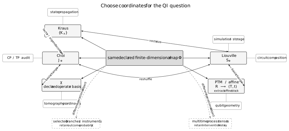
The coordinates change, the declared channel does not. Solid arrows are algebraic conversions after conventions are frozen; dashed exits mark selected operations or instruments and multitime process tensors as different operational objects.

The central map in the figure is a declaration, not an equivalence proof. Solid routes are trustworthy only with the convention record attached. The two dashed exits deliberately leave the coordinate family: conditioning on an outcome changes trace bookkeeping, while resolving a multitime process changes the number and type of intervention slots.

Compose Channels in Circuits

Composition acts right to left

Suppose $\Phi$ acts first and $\Psi$ acts second. States evolve as

$$\rho \longmapsto \Phi(\rho) \longmapsto \Psi[\Phi(\rho)],$$

so the composite is $\Psi\circ\Phi$. In column-stacked Liouville coordinates,

$$S_{\Psi\circ\Phi}=S_\Psi S_\Phi.$$

The rightmost matrix acts first. The same order holds for PTMs. In Kraus coordinates, a family for the composite is $\{L_bK_a\}_{a,b}$ if $\{K_a\}$ represents $\Phi$ and $\{L_b\}$ represents $\Psi$. The family may contain redundant operators and can be compressed by converting through the Choi matrix.

This order convention must be connected to the circuit diagram’s time direction. Some circuit software lists instructions from top to bottom, some displays time left to right, and some accumulates matrices with a left-action or right-action API. A two-operation unit test with noncommuting maps is more reliable than an undocumented phrase such as “in circuit order.” Audit 2 deliberately uses a Hadamard and dephasing because reversing them changes a simple output.

Tensor products, local channels, and subsystem order

Independent local maps act as $\Phi_A\otimes\Psi_B$, but the numerical Kronecker product depends on how operator coordinates order the $A$ and $B$ indices. A library whose state basis is $\lvert a\rangle\otimes\lvert b\rangle$ may still vectorize operators with a different fast index. Build one matrix-unit test, for example $\lvert a b\rangle\!\langle i j\rvert$, and verify where each composite index lands.

Product-channel notation also encodes an independence assumption. A two-qubit crosstalk channel is not generally equal to $\Phi_A\otimes\Phi_B$, even if its single-qubit marginals resemble the factors. Likewise, applying local fitted channels simultaneously can miss correlated coherent phases or shared fluctuations. Tensor factorization should therefore be recorded as a model claim and tested under the simultaneous contexts in which it will be used.

When a channel acts on only part of a larger register, embed it as $\Phi_A\otimes\operatorname{id}_{\bar A}$ in the declared tensor order. Complete positivity guarantees that this extension is physical. An ad hoc positive but non-CP map may appear harmless on isolated $A$ states and fail precisely in this entangled-register use.

Frames, circuit locations, and time dependence

A channel must be placed relative to the ideal gate. “Noise on $U$” could mean $\mathcal N\circ\mathcal U$, $\mathcal U\circ\mathcal N$, or a dressed error $\mathcal U\circ\mathcal E$ in a rotating frame. Those maps are unequal when the noise is anisotropic or nonunital. Record whether a fitted error is in the laboratory frame, the ideal gate’s interaction frame, a Pauli frame, or a compiler-defined logical frame.

Circuit location matters as much as algebraic order. A duration-dependent idle channel, a measurement branch, and a reset map cannot be moved across a gate merely because all are represented by matrices. Classical feedforward composes instruments with conditional later maps, not just unread CPTP sums. Circuit Model owns the ideal syntax, causal order, registers, classical outcomes, and resource accounting; this page owns the representation record attached to each declared channel location.

Time dependence requires an index such as $\Phi_{t,c}$, where $c$ captures context. Replacing a sequence by powers $S^m$ assumes one stationary map applied repeatedly. That approximation can be useful, but drift, control-history dependence, and memory invalidate the algebra even when each one-time estimate is individually CPTP.

Use Channels in Simulation and Inference

Dense propagation and matrix-free application

Dense $S$ makes propagation and composition concise, but its memory cost is $d^4$ complex entries for a square $d$-dimensional system. A complex128 entry occupies 16 bytes. Five qubits require $2^{20}$ entries, or 16 MiB, before temporary arrays; ten qubits require $2^{40}$ entries, or 16 TiB. The dense representation is therefore an audit tool for small systems, not a default scalable data structure.

Matrix-free alternatives apply Kraus operators directly, exploit locality, represent superoperators as tensor networks, or integrate an underlying generator. The appropriate choice depends on Kraus rank, locality, entanglement growth, requested observables, and whether exact density-matrix propagation is necessary. A conversion routine should expose an action interface even when it can also materialize $S$.

Numerical checks need scales and tolerances. Verify trace and Hermiticity after action, but do not repair them silently at every step; repeated renormalization can conceal a TNI/TP mistake. Compare a matrix-free route against a dense reference on small instances and retain the input seed, convention record, and expected output. Noise Simulation owns those algorithms and performance studies.

Random-unitary sampling and Kraus trajectories

For a random-unitary channel $\Phi(\rho)=\sum_ap_aU_a\rho U_a^\dagger$, sampling $a$ with probability $p_a$ and evolving a pure state can estimate ensemble observables without storing a density matrix. The Pauli audit is of this form. Repeated samples reproduce the channel average, while any single trajectory is one realization of the chosen stochastic model.

A general Kraus representation does not automatically supply state-independent probabilities $p_a$. The branch probability is $\operatorname{Tr}(K_a\rho K_a^\dagger)$ and depends on the current state. Sampling then requires computing that probability and normalizing the selected branch. Because Kraus families are nonunique, the resulting trajectory labels are unraveling dependent even though their unread average is the same channel.

This distinction prevents a coordinate artifact from becoming a mechanism claim. A convenient Kraus decomposition can accelerate simulation, but it does not prove that the environment performed the corresponding labeled events. Physical trajectory interpretations require a declared environmental monitoring scheme or stochastic model.

Tomography coordinates are not a validation protocol

Process tomography estimates coordinates from preparation-and-measurement data. The output may be $\chi$, $J$, $R$, or another parameterization, but the representation does not specify which inputs were prepared, which observables were measured, how SPAM was treated, what gauge was fixed, or how uncertainty was propagated. Early prescriptions by Chuang and Nielsen (1997) and Poyatos, Cirac, and Zoller (1997) establish coordinate reconstruction ideas; modern gate-set tomography makes the gauge and self-consistent SPAM problem explicit (Nielsen et al. 2021).

SPAM Errors owns the QI-facing composition of actual preparation maps, intervening processes, effects and instruments, restricted assignment responses, identifiability, and gate-set gauge; this page retains the convention-complete channel-representation dictionary, conversions, composition, and physicality checks.

A constrained estimator may enforce $J\succeq0$ and TP, producing a physical estimate even if raw linear inversion violates them. That is often appropriate, but the constraint is part of the inference model. Report residuals, uncertainty, and held-out predictions rather than using “CPTP” as evidence that the estimate is accurate.

The correct handoff is therefore two-layered: a convention-complete channel record plus a protocol record. Process Tomography owns experimental design, estimators, SPAM assumptions, gauge, uncertainty, and validation; the representation dictionary here lets its outputs enter simulation or circuit analysis without an index change.

When a Single Channel Is Inadequate

Initial correlations and assignment dependence

A reduced map from system input to system output is well defined only relative to how the joint system–environment state is assigned at the input. If the system and environment are initially correlated, independently varying the system state while holding one joint preparation rule may be impossible. Different preparation procedures that yield the same reduced $\rho_S$ can then produce different outputs.

Fitting one channel across those procedures can create apparent non-CP behavior or preparation dependence. The response is not to treat negative Choi eigenvalues as automatically exotic dynamics. First examine the system boundary, preparation map, SPAM model, and whether a common input-output assignment exists. The formal open-system owner develops these caveats; this page only marks the validity condition on the channel record.

Memory, interventions, and process tensors

Repeated use of a fixed channel assumes that the environment is effectively reset or that its retained state does not affect later operations. Temporal correlations violate this assumption. Two sequences can have identical one-time marginals and different responses to an intermediate intervention, so no collection of isolated channel estimates determines the multitime experiment.

A process tensor supplies slots into which control operations are inserted and predicts the resulting terminal statistics. It is a different multilinear object, not an especially large $\chi$ matrix. Pollock et al. (2018) provide a complete operational framework for such non-Markovian processes. A one-use channel remains useful as a marginal or approximation, but it must not be advertised as a context-independent description of memory.

Diagnostic evidence includes history-dependent residuals, failure of a common channel to predict multiple sequence lengths, and changes caused by interventions that leave the immediate reduced input unchanged. Those observations trigger a handoff to multitime/open-system modeling rather than another basis conversion.

Markovian and Non-Markovian Noise owns the operational tests that distinguish one finite map, interval propagation, fixed powers, semigroups, CP divisibility, and multitime memory; this page retains the convention-complete one-use channel dictionary, conversions, composition, and physicality checks.

Leakage, drift, and context transfer

Leakage can make a qubit-only map trace decreasing if population outside the computational subspace is discarded, or CPTP on an enlarged Hilbert space if leakage levels are retained. Both descriptions can be valid, but they answer different questions. The convention record must state the space and whether lost trace is a heralded event, an unobserved level, or physical loss.

Drift creates a family $\Phi_t$, while crosstalk and scheduling create $\Phi_c$. Averaging that family can yield a CPTP channel which predicts mean calibration data yet misses shot correlations or workload dependence. Positivity of the average does not establish stationarity. A claimed transfer should therefore name the tested time window, context set, and observables.

The Noise, Channels, and Error Mitigation guide owns the larger discrepancy–mechanism–evidence–intervention–cost workflow. Here the stopping rule is narrower: if one declared input-output map cannot predict held-out contexts within uncertainty, representation conversion is no longer the bottleneck. Change the operational model or validity domain.

Three Reproducible Finite Audits

The following audits use only small complex arrays and an absolute tolerance of $10^{-12}$. They are intentionally redundant. Each channel is constructed in one representation, converted by independent formulas, and checked by invariants and state action. A hard failure stops execution; a pass prints one line.

Audit 1 — One Pauli channel in five representations

Freeze $p=(0.55,0.15,0.10,0.20)$ in Pauli order $(I,X,Y,Z)$ and set $K_a=\sqrt{p_a}P_a$. In the $P$ basis, $\chi=\operatorname{diag}(0.55,0.15,0.10,0.20)$; in $P/\sqrt2$, it is twice that array. The PTM is

$$R=\operatorname{diag}(1,0.4,0.3,0.5),$$

so the map is TP and unital and sends $(0.6,-0.4,0.2)$ to $(0.24,-0.12,0.10)$. The audit constructs the exact Liouville and Choi arrays, checks their reshuffling difference, verifies the Choi spectrum and partial trace, and applies four representations to the same nontrivial complex state.

Audit 2 — Composition order changes the prediction

Let $\mathcal H$ be Hadamard conjugation and let dephasing contract $X$ and $Y$ by $\eta=0.6$. Starting from $\rho_0=\lvert0\rangle\!\langle0\rvert$,

$$\mathcal D\circ\mathcal H(\rho_0) = \begin{pmatrix}0.5&0.3\\0.3&0.5\end{pmatrix}, \qquad \mathcal H\circ\mathcal D(\rho_0) = \begin{pmatrix}0.5&0.5\\0.5&0.5\end{pmatrix}.$$

Their purities are $0.68$ and $1$, and their trace distance is $0.2$. The audit independently obtains these states from $S_{\mathcal D}S_{\mathcal H}$ and $S_{\mathcal H}S_{\mathcal D}$ and asserts that the superoperators do not commute.

Audit 3 — Instrument branches retain probabilities

Use

$$M_0=\operatorname{diag}(\sqrt{0.9},\sqrt{0.2}), \qquad M_1=\operatorname{diag}(\sqrt{0.1},\sqrt{0.8})$$

on the input state

$$\rho_i= \begin{pmatrix} 0.3&0.1\\ 0.1&0.7 \end{pmatrix}.$$

The effects sum to identity, but neither branch is TP. Their traces are $p_0=0.41$ and $p_1=0.59$. The audit retains both subnormalized branches, checks both conditional states and the unread channel, and proves by direct inequality that branch normalization changed the stored object.

const TOL = 1e-12;
const fail = (m) => { throw new Error(m); };
const check = (q, m) => { if (!q) fail(m); };
const close = (a, b, m) => {
  if (!Number.isFinite(a) || Math.abs(a - b) > TOL) {
    fail(m + ": " + a + " != " + b);
  }
};

const c = (r = 0, i = 0) => [r, i];
const add = (a, b) => c(a[0] + b[0], a[1] + b[1]);
const sub = (a, b) => c(a[0] - b[0], a[1] - b[1]);
const mul = (a, b) =>
  c(a[0] * b[0] - a[1] * b[1], a[0] * b[1] + a[1] * b[0]);
const conj = (a) => c(a[0], -a[1]);
const scale = (a, s) => c(a[0] * s, a[1] * s);
const abs2 = (a) => a[0] * a[0] + a[1] * a[1];

const zeros = (r, s) =>
  Array.from({ length: r }, () =>
    Array.from({ length: s }, () => c())
  );

const eye = (n) =>
  Array.from({ length: n }, (_, i) =>
    Array.from({ length: n }, (_, j) => c(i === j ? 1 : 0))
  );

const mAdd = (a, b) =>
  a.map((row, i) => row.map((x, j) => add(x, b[i][j])));

const mSub = (a, b) =>
  a.map((row, i) => row.map((x, j) => sub(x, b[i][j])));

const mScale = (a, s) =>
  a.map((row) => row.map((x) => scale(x, s)));

const dagger = (a) =>
  a[0].map((_, j) => a.map((row) => conj(row[j])));

const mConj = (a) =>
  a.map((row) => row.map(conj));

const mm = (a, b) =>
  a.map((row) =>
    b[0].map((_, j) =>
      row.reduce(
        (sum, x, k) => add(sum, mul(x, b[k][j])),
        c()
      )
    )
  );

const trace = (a) =>
  a.reduce((sum, row, i) => add(sum, row[i]), c());

const kron = (a, b) => {
  const out = zeros(
    a.length * b.length,
    a[0].length * b[0].length
  );

  for (let i = 0; i < a.length; i++) {
    for (let j = 0; j < a[0].length; j++) {
      for (let r = 0; r < b.length; r++) {
        for (let s = 0; s < b[0].length; s++) {
          out[i * b.length + r][j * b[0].length + s] =
            mul(a[i][j], b[r][s]);
        }
      }
    }
  }

  return out;
};

const outer = (v) =>
  v.map((x) => v.map((y) => mul(x, conj(y))));

const mv = (a, v) =>
  a.map((row) =>
    row.reduce(
      (sum, x, j) => add(sum, mul(x, v[j])),
      c()
    )
  );

const vecCol = (a) => {
  const out = [];

  for (let j = 0; j < a[0].length; j++) {
    for (let i = 0; i < a.length; i++) {
      out.push(a[i][j]);
    }
  }

  return out;
};

const unvecCol = (v, r, s) =>
  Array.from({ length: r }, (_, i) =>
    Array.from({ length: s }, (_, j) => v[i + r * j])
  );

const diag = (v) =>
  v.map((x, i) =>
    v.map((_, j) => c(i === j ? x : 0))
  );

const closeC = (a, b, m) => {
  close(a[0], b[0], m + " re");
  close(a[1], b[1], m + " im");
};

const closeV = (a, b, m) => {
  check(a.length === b.length, m + " length");
  a.forEach((x, i) => closeC(x, b[i], m + "[" + i + "]"));
};

const closeM = (a, b, m) => {
  check(
    a.length === b.length &&
    a[0].length === b[0].length,
    m + " shape"
  );

  a.forEach((row, i) =>
    row.forEach((x, j) =>
      closeC(x, b[i][j], m + "[" + i + "," + j + "]")
    )
  );
};

const maxDiff = (a, b) =>
  Math.max(
    ...a.flatMap((row, i) =>
      row.map((x, j) =>
        Math.hypot(
          x[0] - b[i][j][0],
          x[1] - b[i][j][1]
        )
      )
    )
  );

const apply = (ks, x) =>
  ks.reduce(
    (sum, k) => mAdd(sum, mm(mm(k, x), dagger(k))),
    zeros(ks[0].length, ks[0].length)
  );

const complete = (ks) =>
  ks.reduce(
    (sum, k) => mAdd(sum, mm(dagger(k), k)),
    zeros(ks[0][0].length, ks[0][0].length)
  );

const superop = (ks) =>
  ks.reduce(
    (sum, k) => mAdd(sum, kron(mConj(k), k)),
    zeros(ks[0].length ** 2, ks[0][0].length ** 2)
  );

const choiOI = (ks) =>
  ks.reduce(
    (sum, k) => mAdd(sum, outer(k.flat())),
    zeros(
      ks[0].length * ks[0][0].length,
      ks[0].length * ks[0][0].length
    )
  );

const ptrOut = (j, dOut, dIn) =>
  Array.from({ length: dIn }, (_, i) =>
    Array.from({ length: dIn }, (_, q) => {
      let sum = c();

      for (let a = 0; a < dOut; a++) {
        sum = add(
          sum,
          j[a * dIn + i][a * dIn + q]
        );
      }

      return sum;
    })
  );

const applyChoi = (j, x, dOut, dIn) =>
  Array.from({ length: dOut }, (_, a) =>
    Array.from({ length: dOut }, (_, b) => {
      let sum = c();

      for (let i = 0; i < dIn; i++) {
        for (let q = 0; q < dIn; q++) {
          sum = add(
            sum,
            mul(
              j[a * dIn + i][b * dIn + q],
              x[i][q]
            )
          );
        }
      }

      return sum;
    })
  );

const purity = (rho) => {
  const p = trace(mm(rho, rho));
  close(p[1], 0, "purity imaginary residual");
  return p[0];
};

const traceDistance2 = (a, b) => {
  const d = mSub(a, b);

  close(d[0][0][1], 0, "distance diagonal");
  closeC(
    d[1][0],
    conj(d[0][1]),
    "distance Hermiticity"
  );

  const disc = Math.sqrt(
    (d[0][0][0] - d[1][1][0]) ** 2 +
    4 * abs2(d[0][1])
  );

  const t = d[0][0][0] + d[1][1][0];

  return (
    Math.abs((t + disc) / 2) +
    Math.abs((t - disc) / 2)
  ) / 2;
};

// Audit 1: one Pauli channel in five representations.

const I = [[c(1), c()], [c(), c(1)]];
const X = [[c(), c(1)], [c(1), c()]];
const Y = [[c(), c(0, -1)], [c(0, 1), c()]];
const Z = [[c(1), c()], [c(), c(-1)]];

const P = [I, X, Y, Z];
const p = [0.55, 0.15, 0.10, 0.20];

close(
  p.reduce((s, x) => s + x, 0),
  1,
  "Pauli probability sum"
);
check(
  p.every((x) => x >= 0),
  "negative Pauli probability"
);

const K = P.map(
  (x, i) => mScale(x, Math.sqrt(p[i]))
);

closeM(
  complete(K),
  eye(2),
  "Pauli Kraus completeness"
);

closeM(
  diag(p),
  diag([0.55, 0.15, 0.10, 0.20]),
  "chi in P basis"
);

closeM(
  diag(p.map((x) => 2 * x)),
  diag([1.10, 0.30, 0.20, 0.40]),
  "chi in P/sqrt(2) basis"
);

const R = P.map((a) =>
  P.map((b) => {
    const t = trace(mm(a, apply(K, b)));
    return c(t[0] / 2, t[1] / 2);
  })
);

closeM(
  R,
  diag([1, 0.4, 0.3, 0.5]),
  "Pauli transfer matrix"
);

closeV(
  R[0],
  [c(1), c(), c(), c()],
  "TP first row"
);

closeV(
  R.map((row) => row[0]),
  [c(1), c(), c(), c()],
  "unital first column"
);

const S = superop(K);

closeM(
  S,
  [
    [c(0.75), c(), c(), c(0.25)],
    [c(), c(0.35), c(0.05), c()],
    [c(), c(0.05), c(0.35), c()],
    [c(0.25), c(), c(), c(0.75)]
  ],
  "column-stacked superoperator"
);

const J = choiOI(K);

closeM(
  J,
  [
    [c(0.75), c(), c(), c(0.35)],
    [c(), c(0.25), c(0.05), c()],
    [c(), c(0.05), c(0.25), c()],
    [c(0.35), c(), c(), c(0.75)]
  ],
  "output-input Choi"
);

closeM(
  ptrOut(J, 2, 2),
  eye(2),
  "Choi TP partial trace"
);

closeC(
  trace(J),
  c(2),
  "unnormalized Choi trace"
);

check(
  Math.abs(J[0][3][0] - S[0][3][0]) > TOL,
  "Choi and superoperator conflated"
);

const q = 1 / Math.sqrt(2);

const bell = [
  [c(q), c(), c(), c(q)],
  [c(), c(q), c(q), c()],
  [c(), c(0, -q), c(0, q), c()],
  [c(q), c(), c(), c(-q)]
];

const eig = [1.10, 0.30, 0.20, 0.40];

bell.forEach((v, i) =>
  closeV(
    mv(J, v),
    v.map((x) => scale(x, eig[i])),
    "Choi eigenpair " + i
  )
);

close(
  eig.reduce((s, x) => s + x, 0),
  2,
  "Choi eigenvalue sum"
);

check(
  eig.every((x) => x >= -TOL),
  "Choi is not positive"
);

const rho = [
  [c(0.6), c(0.3, 0.2)],
  [c(0.3, -0.2), c(0.4)]
];

const expectedOut = [
  [c(0.55), c(0.12, 0.06)],
  [c(0.12, -0.06), c(0.45)]
];

closeM(
  apply(K, rho),
  expectedOut,
  "Kraus state action"
);

closeM(
  applyChoi(J, rho, 2, 2),
  expectedOut,
  "Choi state action"
);

closeM(
  unvecCol(mv(S, vecCol(rho)), 2, 2),
  expectedOut,
  "superoperator state action"
);

closeV(
  mv(R, [c(1), c(0.6), c(-0.4), c(0.2)]),
  [c(1), c(0.24), c(-0.12), c(0.10)],
  "PTM Bloch action"
);

// Audit 2: composition order.

const H = mScale(
  [[c(1), c(1)], [c(1), c(-1)]],
  q
);

const KH = [H];
const eta = 0.6;

const KD = [
  mScale(I, Math.sqrt((1 + eta) / 2)),
  mScale(Z, Math.sqrt((1 - eta) / 2))
];

closeM(
  complete(KH),
  eye(2),
  "Hadamard completeness"
);

closeM(
  complete(KD),
  eye(2),
  "dephasing completeness"
);

const SH = superop(KH);
const SD = superop(KD);

closeM(
  SH,
  [
    [c(0.5), c(0.5), c(0.5), c(0.5)],
    [c(0.5), c(-0.5), c(0.5), c(-0.5)],
    [c(0.5), c(0.5), c(-0.5), c(-0.5)],
    [c(0.5), c(-0.5), c(-0.5), c(0.5)]
  ],
  "Hadamard superoperator"
);

closeM(
  SD,
  diag([1, 0.6, 0.6, 1]),
  "dephasing superoperator"
);

const rho0 = [[c(1), c()], [c(), c()]];

const DafterH = apply(KD, apply(KH, rho0));
const HafterD = apply(KH, apply(KD, rho0));

const expectedDafterH = [
  [c(0.5), c(0.3)],
  [c(0.3), c(0.5)]
];

const expectedHafterD = [
  [c(0.5), c(0.5)],
  [c(0.5), c(0.5)]
];

closeM(DafterH, expectedDafterH, "D after H");
closeM(HafterD, expectedHafterD, "H after D");
close(purity(DafterH), 0.68, "D-after-H purity");
close(purity(HafterD), 1, "H-after-D purity");
close(traceDistance2(DafterH, HafterD), 0.2, "order trace distance");

closeM(
  unvecCol(mv(mm(SD, SH), vecCol(rho0)), 2, 2),
  expectedDafterH,
  "S_D S_H"
);

closeM(
  unvecCol(mv(mm(SH, SD), vecCol(rho0)), 2, 2),
  expectedHafterD,
  "S_H S_D"
);

check(
  maxDiff(mm(SD, SH), mm(SH, SD)) > TOL,
  "composition order erased"
);

// Audit 3: instrument branches are not channels.

const M0 = [
  [c(Math.sqrt(0.9)), c()],
  [c(), c(Math.sqrt(0.2))]
];

const M1 = [
  [c(Math.sqrt(0.1)), c()],
  [c(), c(Math.sqrt(0.8))]
];

closeM(
  complete([M0, M1]),
  eye(2),
  "instrument completeness"
);

const ri = [
  [c(0.3), c(0.1)],
  [c(0.1), c(0.7)]
];

const b0 = mm(mm(M0, ri), dagger(M0));
const b1 = mm(mm(M1, ri), dagger(M1));

const p0 = trace(b0);
const p1 = trace(b1);

closeC(p0, c(0.41), "p0");
closeC(p1, c(0.59), "p1");
close(p0[0] + p1[0], 1, "branch probability sum");

closeM(
  b0,
  [
    [c(0.27), c(3 / (50 * Math.sqrt(2)))],
    [c(3 / (50 * Math.sqrt(2))), c(0.14)]
  ],
  "branch 0"
);

closeM(
  b1,
  [
    [c(0.03), c(1 / (25 * Math.sqrt(2)))],
    [c(1 / (25 * Math.sqrt(2))), c(0.56)]
  ],
  "branch 1"
);

const c0 = mScale(b0, 1 / p0[0]);
const c1 = mScale(b1, 1 / p1[0]);

closeM(
  c0,
  [
    [c(27 / 41), c(3 * Math.sqrt(2) / 41)],
    [c(3 * Math.sqrt(2) / 41), c(14 / 41)]
  ],
  "conditional 0"
);

closeM(
  c1,
  [
    [c(3 / 59), c(2 * Math.sqrt(2) / 59)],
    [c(2 * Math.sqrt(2) / 59), c(56 / 59)]
  ],
  "conditional 1"
);

closeC(trace(c0), c(1), "conditional 0 trace");
closeC(trace(c1), c(1), "conditional 1 trace");

closeM(
  mAdd(b0, b1),
  [
    [c(0.3), c(1 / (10 * Math.sqrt(2)))],
    [c(1 / (10 * Math.sqrt(2))), c(0.7)]
  ],
  "unread channel"
);

closeC(
  trace(mm(mm(dagger(M0), M0), ri)),
  p0,
  "effect probability 0"
);

closeC(
  trace(mm(mm(dagger(M1), M1), ri)),
  p1,
  "effect probability 1"
);

check(
  maxDiff(mm(dagger(M0), M0), eye(2)) > TOL,
  "branch 0 incorrectly treated as TP"
);

check(
  maxDiff(mm(dagger(M1), M1), eye(2)) > TOL,
  "branch 1 incorrectly treated as TP"
);

check(
  Math.abs(p0[0] - 1) > TOL,
  "branch probability erased"
);

check(
  maxDiff(b0, c0) > TOL,
  "branch and conditional state conflated"
);

console.log("Quantum-channels-for-QI finite audits: PASS");

The first audit’s exact Choi eigenvalues are $\{1.10,0.30,0.20,0.40\}$ in the Bell vectors associated with $(I,X,Y,Z)$, and their sum is the unnormalized Choi trace $2$. The third audit yields

$$\widetilde\rho_0= \begin{pmatrix}0.27&3/(50\sqrt2)\\3/(50\sqrt2)&0.14\end{pmatrix}, \qquad \widetilde\rho_1= \begin{pmatrix}0.03&1/(25\sqrt2)\\1/(25\sqrt2)&0.56\end{pmatrix},$$

whose sum has coherence $1/(10\sqrt2)$. These values are useful fixtures because they detect normalization, index-order, complex-conjugation, and premature-branch-normalization errors with one small example.

Canonical Owners and Chapter Routes

Channel work crosses several subjects, but each question has one canonical owner. Use this page for finite-dimensional representation choice, conversion, composition, and checks. Follow the table when the question changes from coordinates to states, formal theorems, mechanisms, circuits, model cards, numerical algorithms, or inference protocols.

Kraus, Choi, and Stinespring Views owns the focused unread-map equivalence, minimal Kraus–Choi–Stinespring realization, compression, and environment-record crosswalk; this page retains the broader convention ledger, representation selection and conversion, physicality checks, circuit composition, and simulation and inference workflow.

Question	Canonical owner	Retained scope
How are mixed states, ensembles, marginals, purifications, and subnormalized branches represented?	Density Operators for Quantum Information	state bookkeeping rather than channel-coordinate conversion
Why are channels CP, how do representation and dilation theorems work, and what are operations or instruments?	Quantum Channels and Noise	definitions, proofs, Stinespring theory, fixed points, generators, and open-system scope
How does a discrepancy become a model, evidence test, intervention, and cost record?	Noise, Channels, and Error Mitigation	chapter-level decision and evidence workflow
What do circuit wires, operation order, registers, outcomes, and resource counts mean?	Circuit Model	ideal syntax, causal semantics, classical control, and logical resources
Which physical or operational mechanisms can produce observed errors?	Noise in Quantum Information	mechanism taxonomy, context, accumulation, diagnostics, and engineering consequences
Which standard channel card and parameter convention should model a device?	Common Noise Models	explicit models, placement rules, conversions, and falsifiers
How should a Pauli law be composed, propagated through Clifford structure, or pushed to syndrome and logical classes?	Pauli Noise and Depolarizing Channels	Pauli probabilities, transfer eigenvalues, depolarizing conventions, stabilizer propagation, and approximation limits
How should a qualified T1–T2 and equilibrium-population record become a physical, composable idle channel?	Dephasing and Amplitude Damping	Protocol-qualified relaxation and coherence conversion, thermal translation, physicality, composition, and held-out checks
How should computational-sector leakage, seepage, survival branches, flags, and context-dependent subsystem errors be modeled and falsified?	Leakage and Crosstalk	Full-space versus retained processes, leakage and coherent-return diagnostics, scalar population licenses, operational crosstalk tests, and context-aware composition
How is a learned signed inverse-channel decomposition constructed, sampled, and validated?	Probabilistic Error Cancellation	implemented-basis QPD and estimator reconstruction rather than general representation, conversion, composition, or physicality theory
How should a channel be applied scalably and cross-validated numerically?	Noise Simulation	algorithms, matrix-free execution, trajectories, performance, and uncertainty sampling
How are channel coordinates estimated from experiments and validated out of sample?	Process Tomography	designs, estimators, SPAM, gauge, uncertainty, and holdout tests

This routing preserves canonical homes while allowing a complete QI workflow. In particular, the planned deeper representation leaf is not used as an owner until it is promoted. For a standard broad reference connecting channels to quantum computation, Nielsen and Chuang (2010) remains a useful entry point; the formal and operational boundaries above determine where this site’s derivations live.

Common Channel-Representation Failures

Calling every CP map a channel. A selected branch is usually CP-TNI, not TP. Keep its trace as the event probability, and call an outcome-indexed family an instrument. Only the unread sum is a deterministic channel when its effects are complete.

Treating Choi normalization as universal. This page uses an unnormalized Choi matrix with trace $d_{\mathrm{in}}$ for TP maps. If another source uses a normalized entangled state, translate the factor before comparing spectra, traces, or process fidelities.

Equating Choi and Liouville arrays. They share four-index data but pair the indices differently. Apply $(J_\Phi)_{ai,bj}=(S_\Phi)_{ab,ij}$ as a reshuffle. A direct array equality is generally false even for a simple Pauli channel.

Leaving vec undefined. Column stacking gives $S=\sum K^*\otimes K$; row stacking gives another ordering. A file format or API must declare which convention it uses and should include a small matrix-unit fixture.

Forgetting operator-basis normalization. A $\chi$ matrix changes when $P$ is replaced by $P/\sqrt2$. The map is unchanged. Comparing $\chi$ entries without the ordered basis can manufacture a factor-of-two discrepancy or a sign error in the $Y$ component.

Reading Kraus labels as physical events. Kraus families are related by isometries on their label space. A label becomes an event only after an instrument or environmental monitoring model gives it operational meaning.

Reversing circuit order. If $\Phi$ acts first and $\Psi$ second, the Liouville product is $S_\Psi S_\Phi$. Test a noncommuting pair and name the frame and circuit location rather than relying on an ambiguous multiplication convention.

Using PTM row and column checks as CP certification. The first row checks TP and the first column checks unitality under this convention. Neither prevents a negative Choi eigenvalue. Convert or reshuffle to the declared Choi representation for the CP test.

Converting coordinates into a mechanism claim. Choi positivity, an affine translation, or a diagonal $\chi$ establishes properties of a fitted map, not a microscopic cause, stationarity, locality, or context transfer. Those claims need independent physical and experimental evidence.

Calling a one-use process matrix a process tensor. A $\chi$ matrix coordinates one map. A process tensor predicts sequences of interventions and retains temporal correlations. Missing multitime data cannot be created by a basis conversion.

Exercises

1. Test a dephasing Choi family

For real $t$, consider

$$J_t= \begin{pmatrix} 1&0&0&t\\ 0&0&0&0\\ 0&0&0&0\\ t&0&0&1 \end{pmatrix}.$$

Determine when it defines a CPTP map under this page’s Choi convention. Test unitality, find its spectrum and a Kraus family, and give its PTM.

Solution

Tracing over the output gives $I$ for every real $t$, so the represented map is TP whenever it is CP. Tracing over the input also gives $I$, so it is unital. The only nonzero block is

$$\begin{pmatrix}1&t\\t&1\end{pmatrix},$$

with eigenvalues $1+t$ and $1-t$ and normalized eigenvectors $(\lvert00\rangle\pm\lvert11\rangle)/\sqrt2$. The other two eigenvalues are zero. Hence $J_t\succeq0$ exactly when $|t|\le1$.

Reshaping the two weighted eigenvectors gives the Kraus family

$$K_0=\sqrt{\frac{1+t}{2}}I, \qquad K_1=\sqrt{\frac{1-t}{2}}Z.$$

The weights are nonnegative precisely in the CP interval and sum to one. Conjugation by $I$ leaves every Pauli component fixed, while conjugation by $Z$ reverses $X$ and $Y$. Therefore

$$R=\operatorname{diag}(1,t,t,1).$$

At $t=1$ the map is identity; at $t=-1$ it is $Z$ conjugation; and at $t=0$ it completely dephases in the computational basis.

2. Convert one Pauli channel five ways

Starting from $(p_I,p_X,p_Y,p_Z)=(0.55,0.15,0.10,0.20)$, reproduce the Kraus, $\chi$, PTM, Liouville, and output–input Choi representations. Include both $\chi$ normalizations, the Choi eigenpairs and partial trace, and the output on the audit state.

Solution

Take $K_a=\sqrt{p_a}P_a$. Since $P_a^\dagger P_a=I$ and $\sum_ap_a=1$, the family is complete. In the unnormalized Pauli basis,

$$\chi_P=\operatorname{diag}(0.55,0.15,0.10,0.20),$$

whereas in $P/\sqrt2$ the matrix is

$$\chi_{P/\sqrt2}=2\chi_P =\operatorname{diag}(1.10,0.30,0.20,0.40).$$

Pauli conjugation gives contractions $p_I+p_X-p_Y-p_Z=0.4$ on $X$, $p_I-p_X+p_Y-p_Z=0.3$ on $Y$, and $p_I-p_X-p_Y+p_Z=0.5$ on $Z$. Thus $R=\operatorname{diag}(1,0.4,0.3,0.5)$.

Column stacking and output–input Choi ordering give

$$S= \begin{pmatrix} 0.75&0&0&0.25\\ 0&0.35&0.05&0\\ 0&0.05&0.35&0\\ 0.25&0&0&0.75 \end{pmatrix},$$ $$J= \begin{pmatrix} 0.75&0&0&0.35\\ 0&0.25&0.05&0\\ 0&0.05&0.25&0\\ 0.35&0&0&0.75 \end{pmatrix}.$$

The Bell vectors associated with $(I,X,Y,Z)$ have eigenvalues $(1.10,0.30,0.20,0.40)$. They are nonnegative, sum to $2$, and $\operatorname{Tr}_{\mathrm{out}}J=I$. Direct Kraus action, Choi contraction, $S\operatorname{vec}_{\mathrm{col}}(\rho)$, and PTM action all give

$$\Phi(\rho)= \begin{pmatrix} 0.55&0.12+0.06i\\ 0.12-0.06i&0.45 \end{pmatrix}.$$

The five arrays are different coordinates of the same map because all invariant and action checks agree.

3. Reshuffle rather than relabel

Starting from the Audit 1 superoperator, reconstruct the output–input Choi matrix using $(J_\Phi)_{ai,bj}=(S_\Phi)_{ab,ij}$. Explain why this is not direct equality and verify the entries $J_{03}$ and $S_{03}$.

Solution

Interpret each Liouville row as a pair $(a,b)$ and each column as $(i,j)$. Move the middle indices so that the Choi row is $(a,i)$ and its column is $(b,j)$. Index explicitly as J[a*dIn+i][b*dIn+j] = S[a+dOut*b][i+dIn*j]. Equivalently, a row-major reshape views $S$ with axes $(b,a,j,i)$, which are transposed to $(a,i,b,j)$; a column-major reshape uses $(a,b,i,j)\to(a,i,b,j)$.

For Choi entry $(0,3)$, the composite indices are $(a,i)=(0,0)$ and $(b,j)=(1,1)$. The corresponding Liouville entry is row $(a,b)=(0,1)$ and column $(i,j)=(0,1)$, which carries $0.35$. Hence $J_{03}=0.35$. By contrast, $S_{03}$ directly means row $(a,b)=(0,0)$ and column $(i,j)=(1,1)$, and equals $0.25$.

The mismatch is expected: reshuffling changes which elementary indices are paired into a row and column. Applying the inverse reshuffle recovers $S$, so no information was lost. Testing $J=S$ would confuse coordinate layout with channel equality.

4. Compose dephasing and a Hadamard

For $\eta=0.6$ and input $\lvert0\rangle\!\langle0\rvert$, compute dephasing after a Hadamard and a Hadamard after dephasing. Find both purities, their trace distance, and the corresponding superoperator products.

Solution

Hadamard first produces $\lvert+\rangle\!\langle+\rvert$. Dephasing preserves its populations and multiplies its off-diagonal entries by $0.6$, so

$$\mathcal D\circ\mathcal H(\rho_0) = \begin{pmatrix}0.5&0.3\\0.3&0.5\end{pmatrix}.$$

Dephasing first leaves the computational-basis state $\rho_0$ unchanged; Hadamard then produces the pure plus state,

$$\mathcal H\circ\mathcal D(\rho_0) = \begin{pmatrix}0.5&0.5\\0.5&0.5\end{pmatrix}.$$

For the first matrix, $\operatorname{Tr}(\rho^2)=2(0.5^2)+2(0.3^2)=0.68$. The second is a rank-one projector and has purity one. Their difference has eigenvalues $\pm0.2$, so half its trace norm is $0.2$.

Because the rightmost operation acts first, the first result is generated by $S_{\mathcal D}S_{\mathcal H}$ and the second by $S_{\mathcal H}S_{\mathcal D}$. The products are unequal. This concrete output difference is the required unit test for a circuit-order convention.

5. Retain instrument probabilities

Apply the two diagonal instrument operators from Audit 3 to $\rho_i$. Compute both subnormalized branches, probabilities, conditional states, and the unread channel. State exactly what premature normalization erases.

Solution

Direct multiplication gives

$$\widetilde\rho_0= \begin{pmatrix} 0.27&3/(50\sqrt2)\\ 3/(50\sqrt2)&0.14 \end{pmatrix}, \qquad p_0=0.41,$$

and

$$\widetilde\rho_1= \begin{pmatrix} 0.03&1/(25\sqrt2)\\ 1/(25\sqrt2)&0.56 \end{pmatrix}, \qquad p_1=0.59.$$

The probabilities sum to one because $M_0^\dagger M_0+M_1^\dagger M_1=I$. Dividing each branch by its own trace yields

$$\rho_{0\mid0}= \begin{pmatrix} 27/41&3\sqrt2/41\\ 3\sqrt2/41&14/41 \end{pmatrix},$$ $$\rho_{1\mid1}= \begin{pmatrix} 3/59&2\sqrt2/59\\ 2\sqrt2/59&56/59 \end{pmatrix}.$$

If the result is unread, sum before normalization:

$$\rho'=\begin{pmatrix} 0.3&1/(10\sqrt2)\\ 1/(10\sqrt2)&0.7 \end{pmatrix}.$$

Replacing $\widetilde\rho_y$ immediately by $\rho_{y\mid y}$ sets every stored trace to one. It erases $p_y$, so later code cannot reproduce outcome frequencies, likelihoods, or correctly weighted feedforward branches.

6. Change the process-matrix basis

Rewrite the Audit 1 Pauli channel from basis $P=(I,X,Y,Z)$ to $P/\sqrt2$. Derive the transformed $\chi$, show that the map is unchanged, and distinguish the result from a process tensor.

Solution

Let $A_m=P_m$ and $A'_m=P_m/\sqrt2$. Each term in the process expansion changes according to

$$A'_m\rho A_n'^\dagger =\frac12A_m\rho A_n^\dagger.$$

To preserve the sum, the coordinate matrix must therefore change as $\chi'=2\chi$. Thus

$$\chi'= \operatorname{diag}(1.10,0.30,0.20,0.40).$$

Substitution gives

$$\sum_m\chi'_{mm}A'_m\rho A_m'^\dagger = \sum_mp_mP_m\rho P_m,$$

which is the original channel. Its Choi matrix, PTM, state action, and physicality properties are unchanged because only coordinates changed.

Both $\chi$ arrays describe one input-output map at one declared use. A process tensor instead accepts a sequence of interventions and retains temporal correlations. No basis rescaling can supply those additional slots or the multitime data required to identify them.

7. Propagate an observable backward

For the Audit 1 channel and $A=0.2I+0.4X-0.3Y+0.5Z$, find $\Phi^\dagger(A)$. Verify forward and backward expectation values on the audit input state.

Solution

The Pauli channel is self-adjoint in the Hilbert–Schmidt inner product because each Pauli is Hermitian and the weights are real. Its adjoint has the same Pauli contractions $(0.4,0.3,0.5)$. Therefore

$$\Phi^\dagger(A) =0.2I+0.16X-0.09Y+0.25Z.$$

The output state’s Bloch vector is $\boldsymbol r'=(0.24,-0.12,0.10)$. For $A=a_0I+\boldsymbol a\cdot\boldsymbol\sigma$, the expectation is $a_0+\boldsymbol a\cdot\boldsymbol r'$, giving

$$0.2+0.4(0.24)-0.3(-0.12)+0.5(0.10)=0.382.$$

Using the original input vector $(0.6,-0.4,0.2)$ with the adjoint coefficients gives

$$0.2+0.16(0.6)-0.09(-0.4)+0.25(0.2)=0.382.$$

Hence $\operatorname{Tr}[A\Phi(\rho)]=\operatorname{Tr}[\Phi^\dagger(A)\rho]$ in the explicit fixture. Agreement checks the PTM orientation as well as the adjoint action.

8. Price a full superoperator

For an $n$-qubit channel with equal input and output spaces, compute the number of entries and complex128 storage of a dense Liouville superoperator. Evaluate the result at five and ten qubits and identify the appropriate handoff for scalable execution.

Solution

The Hilbert-space dimension is $d=2^n$. Liouville space has dimension $d^2$, so a square dense superoperator contains

$$d^4=(2^n)^4=2^{4n}$$

complex entries. Complex128 stores 16 bytes per entry before allocator overhead, decompositions, or scratch arrays.

At five qubits, $2^{20}$ entries require $2^{24}$ bytes, exactly 16 MiB. At ten qubits, $2^{40}$ entries require $2^{44}$ bytes, exactly 16 TiB. Increasing the register from five to ten qubits multiplies storage by $2^{20}$.

These figures exclude temporary matrices used in composition, eigendecomposition, or reshuffling. Large-system work should use matrix-free Kraus action, locality, tensor-network structure, trajectories, or another problem-specific representation. Noise Simulation is the canonical owner for choosing and validating those scalable algorithms.

References

• M.-D. Choi, “Completely Positive Linear Maps on Complex Matrices,” Linear Algebra and its Applications 10, 285–290 (1975), doi:10.1016/0024-3795(75)90075-0.
• I. L. Chuang and M. A. Nielsen, “Prescription for Experimental Determination of the Dynamics of a Quantum Black Box,” Journal of Modern Optics 44, 2455–2467 (1997), doi:10.1080/09500349708231894.
• A. Gilchrist, N. K. Langford, and M. A. Nielsen, “Distance Measures to Compare Real and Ideal Quantum Processes,” Physical Review A 71, 062310 (2005), doi:10.1103/PhysRevA.71.062310.
• T. F. Havel, “Robust Procedures for Converting among Lindblad, Kraus and Matrix Representations of Quantum Dynamical Semigroups,” Journal of Mathematical Physics 44, 534–557 (2003), doi:10.1063/1.1518555.
• A. S. Holevo and V. Giovannetti, “Quantum Channels and Their Entropic Characteristics,” Reports on Progress in Physics 75, 046001 (2012), doi:10.1088/0034-4885/75/4/046001.
• A. Jamiołkowski, “Linear Transformations Which Preserve Trace and Positive Semidefiniteness of Operators,” Reports on Mathematical Physics 3, 275–278 (1972), doi:10.1016/0034-4877(72)90011-0.
• K. Kraus, “General State Changes in Quantum Theory,” Annals of Physics 64, 311–335 (1971), doi:10.1016/0003-4916(71)90108-4.
• E. Nielsen, J. K. Gamble, K. Rudinger, T. Scholten, K. Young, and R. Blume-Kohout, “Gate Set Tomography,” Quantum 5, 557 (2021), doi:10.22331/q-2021-10-05-557.
• M. A. Nielsen and I. L. Chuang, Quantum Computation and Quantum Information, 10th anniversary ed., Cambridge University Press (2010), doi:10.1017/CBO9780511976667.
• F. A. Pollock, C. Rodríguez-Rosario, T. Frauenheim, M. Paternostro, and K. Modi, “Non-Markovian Quantum Processes: Complete Framework and Efficient Characterization,” Physical Review A 97, 012127 (2018), doi:10.1103/PhysRevA.97.012127.
• J. F. Poyatos, J. I. Cirac, and P. Zoller, “Complete Characterization of a Quantum Process: The Two-Bit Quantum Gate,” Physical Review Letters 78, 390–393 (1997), doi:10.1103/PhysRevLett.78.390.
• M. B. Ruskai, S. Szarek, and E. Werner, “An Analysis of Completely-Positive Trace-Preserving Maps on M2,” Linear Algebra and its Applications 347, 159–187 (2002), doi:10.1016/S0024-3795(01)00547-X.
• W. F. Stinespring, “Positive Functions on C*-Algebras,” Proceedings of the American Mathematical Society 6, 211–216 (1955), doi:10.1090/S0002-9939-1955-0069403-4.
• E. C. G. Sudarshan, P. M. Mathews, and J. Rau, “Stochastic Dynamics of Quantum-Mechanical Systems,” Physical Review 121, 920–924 (1961), doi:10.1103/PhysRev.121.920.
• J. Watrous, The Theory of Quantum Information, Cambridge University Press (2018), doi:10.1017/9781316848142.
• C. J. Wood, J. D. Biamonte, and D. G. Cory, “Tensor Networks and Graphical Calculus for Open Quantum Systems,” Quantum Information and Computation 15, 759–811 (2015), doi:10.26421/QIC15.9-10-3.