Probabilistic Error Cancellation

Probabilistic error cancellation (PEC) estimates an ideal observable by sampling physical circuit variants with ordinary positive probabilities and then combining their outcomes with signed weights. The central identity is linear, but its scientific license is demanding: the ideal map must lie in the real span of operations that the device can actually implement, their noise and circuit placement must match the learned model, and the resulting coefficient growth must fit a finite validation and resource budget. When any of those conditions fails, the correct result can be a narrower biased claim, a redesigned basis, or no cancellation at all.

Required background. Error Mitigation Overview supplies the frozen estimand, executable baseline, validation split, combination order, and complete resource ledger. Quantum Channels for QI supplies channel composition, representation, invertibility, and physicality conventions used to define the implemented maps.

Helpful background. Variance and Covariance supplies full-covariance propagation and allocation language, while Kraus, Choi, and Stinespring Views supplies equivalent channel descriptions and the boundary between a physical map and its formal inverse.

Probabilistic Error Cancellation Is Signed Channel Inversion

What this specialist page owns

PEC belongs to the family of estimator-level mitigation methods introduced for short noisy circuits by Temme, Bravyi, and Gambetta (2017) and developed into a practical framework by Endo, Benjamin, and Li (2018). It does not make an unphysical inverse channel occur in one execution. Instead, it represents an ideal operation or inverse noise action as a real linear combination of physical implementations. Each execution selects one term with a positive probability; the classical record restores the coefficient’s sign and scale.

This page owns that construction from end to end: the target and operation order, the implemented basis, exact or approximate quasiprobability decomposition (QPD), sampling law, conditional-unbiasedness proof, coefficient one-norm, variance, learned-model uncertainty, held-out tests, and stop decision. The chapter guide owns the earlier choice among mitigation families. Device characterization, algorithm pages, reporting, lower bounds, error correction, and fault tolerance retain their own questions. A PEC calculation should therefore end with a scoped expectation-value claim and an auditable resource record, not with a claim that the physical output state was repaired.

Freeze the estimand and executable baseline

Let $\rho$ be the declared input, $\mathcal C_{\mathrm{id}}$ the complete ideal circuit channel, and $O$ a Hermitian observable. The target is

$$\mu_{\mathrm{id}} = \operatorname{Tr} [O\,\mathcal C_{\mathrm{id}}(\rho)].$$

Freeze the circuit and observable versions, native gates or pulses, compiler settings, layout, outcome normalization, measurement-response treatment, acceptance rule, calibration epoch, and unmitigated estimate before fitting the noise model or choosing a decomposition. The target is not merely “the answer with less noise”: changing a compiler pass, readout correction, accepted outcome set, or normalization can change the mathematical estimand.

Write one explicit index map from each sampled record to its circuit instance, locationwise basis choices, signed weight, model version, epoch, acceptance status, and raw outcome before aggregation. That record makes it possible to replay an estimate, separate issued from accepted executions, and test whether drift or a basis choice is confounded with the result. Preserve the raw unmitigated baseline and all attempted mitigation settings alongside the final estimate.

Invert maps, not measurement data

A noisy physical channel is completely positive, whereas its linear inverse, when it exists, is usually not. PEC exploits linearity without pretending that the inverse is itself a physical operation. If

$$\mathcal N^{-1} = \sum_a q_a\mathcal B_a, \qquad q_a\in\mathbb R,$$

the $\mathcal B_a$ are implementable maps and the $q_a$ are classical coefficients. Negative $q_a$ values are not negative probabilities. The positive sampling distribution is built from $|q_a|$; the sign reappears only in the weighted outcome.

This channel algebra is distinct from terminal measurement-response inversion. A response matrix maps ideal outcome probabilities to recorded outcomes, whereas a gate-noise map acts during the circuit. Combining the two can be valid, but only after the complete acquisition-to-estimate map and its order are declared. It is not licensed by giving both transformations the word “inverse.”

Freeze the Target, Noise Placement, and Implemented Basis

Declare circuit order and noise orientation

Write the ideal circuit using one explicit convention,

$$\mathcal C_{\mathrm{id}} = \mathcal U_L\circ\cdots\circ\mathcal U_1,$$

so $\mathcal U_1$ acts first. Suppose the physical implementation at location $\ell$ is modeled as noise after the ideal gate,

$$\widetilde{\mathcal U}_\ell = \mathcal N_\ell\circ\mathcal U_\ell.$$

Then the corresponding inverse action belongs after that noisy implementation:

$$\mathcal N_\ell^{-1} \circ \widetilde{\mathcal U}_\ell = \mathcal U_\ell.$$

Moving it before $\mathcal U_\ell$ generally produces $\mathcal N_\ell\circ\mathcal U_\ell\circ\mathcal N_\ell^{-1}$, which need not equal $\mathcal U_\ell$. A before-gate convention can also be used, but it defines a different decomposition. Gate dependence, simultaneous operations, idle intervals, and control history require location and context labels rather than one transferable noise map.

Treat basis operations as implemented maps

An experimentally available basis element is the map realized by a complete physical circuit variant, including the noise on any inserted or replacement gate. An ideal Pauli conjugation written on paper is not automatically that map. If a sampled $X$ correction is itself noisy, its characterized physical implementation—not the noiseless operation $\rho\mapsto X\rho X$—belongs in the decomposition matrix.

The algebraic bit-flip fixtures below license the identity and $X$ branches as exact characterized implemented maps, for example exact virtual Pauli-frame updates whose action is the declared conjugation. This is a fixture assumption, not a claim that arbitrary physical Pauli pulses are noiseless. Every reported “inverse” value in those fixtures is a formal signed-estimator expectation, not the output of a physically executed inverse channel.

Ordinary PEC uses trace-preserving completely positive basis maps. A conditioned instrument or trace-decreasing branch can be admitted only with an explicit outcome, survival normalization, and issued-versus-accepted cost. The same restriction applies to resets, measurements, feedforward, and leakage flags. Hiding them inside a nominal gate name makes the linear identity unreproducible.

Attach context, epoch, and calibration versions

The record for $\mathcal B_{\ell a}$ should name the qubits, neighboring activity, direction, control schedule, compiler output, calibration version, time window, and any twirl or randomization distribution. A map learned on an isolated two-qubit gate may not describe the same pulse executed beside a busy spectator, at a different depth, or after thermal population accumulates.

Context is part of the mathematical object, not optional provenance. If a single fitted map is asserted across contexts, validate that restriction on held-out data. Otherwise use $\mathcal B_{\ell a,c,e}$ with context $c$ and epoch $e$, and keep the science execution inside the supported domain. Calibration uncertainty and drift are propagated later rather than erased by choosing one best-fit version.

Test linear-span and invertibility conditions

Choose a declared Liouville or Pauli-transfer convention, vectorize the target map as $t_\ell$, and stack feasible implemented basis maps as columns of $B_\ell$. The exact problem is

$$B_\ell q_\ell=t_\ell.$$

Inspect rank, singular values, numerical conditioning, equality residual, and coefficient sensitivity. A square fitted noise matrix can be invertible while the feasible basis fails to span its inverse. Conversely, an overcomplete basis can admit many solutions with very different signed norms. Physicality belongs to the basis maps; the target inverse need only be a real linear map on the declared space.

Record	Ideal object	Implemented representation	Coefficient or parameter	Sampling rule	Validation evidence	Stop rule
Target	$\mu_{\mathrm{id}}$ and $\mathcal C_{\mathrm{id}}$	frozen circuit, observable, and normalization	circuit and observable versions	none yet	ideal simulation or trusted reference	target changed after freezing
Noise placement	ordered $\mathcal U_\ell$ locations	before- or after-gate map with context	placement convention	preserve time order	identity and known-answer circuits	placement is ambiguous
Basis element	feasible physical operation	characterized $\mathcal B_{\ell a}$	map estimate and uncertainty	sample only executable variants	held-out basis-operation probes	abstract map replaces implementation
QPD	exact or approximate target equality	$B_\ell q_\ell=t_\ell$	signed $q_{\ell a}$	$	q	/\gamma$ with restored sign
Model version	declared $\mathcal N_{\ell,c,e}$	data, solver, constraints, and epoch	$\widehat\theta$ and covariance	freeze before science holdout	independent predictive checks	version or epoch mismatch
Context	science-domain location and workload	qubits, neighbors, schedule, depth, and twirl	context labels	sample within supported domain	matched circuits and sentinels	unsupported transfer is required
Residual	zero for exact cancellation	$\Delta$ or $\mathcal R_\ell$	norm or empirical discrepancy	no hidden resampling	held-out bias bound	residual exceeds frozen budget

Construct Exact or Approximate Quasiprobability Decompositions

Expand the ideal operation or inverse channel

There are two common but convention-sensitive forms. With after-gate noise one may expand the inverse,

$$\mathcal N_\ell^{-1} = \sum_a q_{\ell a}\mathcal B_{\ell a},$$

and compose each physical correction after $\widetilde{\mathcal U}_\ell$. Alternatively, one may directly decompose the ideal gate into fully implemented variants,

$$\mathcal U_\ell = \sum_a q_{\ell a} \widetilde{\mathcal O}_{\ell a}.$$

The two forms agree only when the maps, physical noise, and side of composition are translated consistently. Direct decomposition can be clearer because each $\widetilde{\mathcal O}_{\ell a}$ is the complete circuit fragment actually run. Inverse-channel notation can be more compact for a reusable noise model. Neither form licenses inserting an ideal basis element whose physical noise was omitted.

Minimize the coefficient one-norm

For an exact feasible decomposition define

$$\gamma_\ell = \lVert q_\ell\rVert_1 = \sum_a|q_{\ell a}|.$$

An overcomplete basis invites the optimization

$$\min_{q_\ell}\lVert q_\ell\rVert_1 \quad\text{subject to}\quad B_\ell q_\ell=t_\ell.$$

Piveteau, Sutter, and Woerner (2022) formulate noise-aware optimization and an approximate variant that trades representation error against sampling cost. Report the representation, feasible operation set, solver, tolerances, constraints, residual, and calibration version. A smaller norm is useful only inside the same licensed target and physical basis; changing the basis model can make a deceptively cheap but wrong decomposition.

For trace-preserving basis maps that sum to a trace-preserving target, $\sum_aq_{\ell a}=1$, so $\gamma_\ell\ge1$. Equality means a nonnegative mixture in that decomposition. Values above one measure signed cancellation, not channel infidelity by themselves.

Quantify approximation residuals

If exact equality is infeasible or unaffordable, write the residual rather than silently regularizing it away:

$$\mathcal C_{\mathrm{id}} = \sum_aq_a\widetilde{\mathcal C}_a+\Delta.$$

For normalized $\rho$ and bounded $O$,

$$\left| \operatorname{Tr}[O\,\Delta(\rho)] \right| \le \lVert O\rVert_\infty \lVert\Delta(\rho)\rVert_1 \le \lVert O\rVert_\infty \lVert\Delta\rVert_\diamond.$$

Here the diamond norm uses the full induced trace norm, without a hidden factor of one half. A state- and observable-specific held-out discrepancy can support a much narrower bound at lower cost; it is not a uniform claim over all inputs and ancillas. Predeclare the bias budget and tradeoff family on training and validation data, then reserve the final holdout for evaluation.

Keep coefficient signs and normalization explicit

For each nonzero term set

$$p_{\ell a} = \frac{|q_{\ell a}|}{\gamma_\ell}, \qquad s_{\ell a} = \operatorname{sgn}(q_{\ell a}).$$

Verify $\sum_ap_{\ell a}=1$ and $q_{\ell a}=\gamma_\ell p_{\ell a}s_{\ell a}$ at full precision. Exact zero coefficients are removed rather than assigned an arbitrary sign. Round values only for display; preserve the full decomposition artifact used for sampling.

This separation prevents a recurring category error. The device samples a valid circuit from the positive law $p_{\ell a}$. The analysis attaches a possibly negative scalar $s_{\ell a}\gamma_\ell$ to its outcome. No run has negative probability, and the weighted record is not distributed like a measurement of the ideal state even when its expectation is correct.

Sample Circuits and Recover the Ideal Expectation

Sample absolute coefficients

For a circuit-level decomposition

$$\mathcal C_{\mathrm{id}} = \sum_aq_a\widetilde{\mathcal C}_a, \qquad \gamma=\sum_a|q_a|,$$

draw $A$ with $p_a=|q_a|/\gamma$, execute $\widetilde{\mathcal C}_A$, and retain its raw bounded measurement outcome $o$. Define the signed record and sample mean by

$$X = \gamma\operatorname{sgn}(q_A)o, \qquad \widehat\mu_{\mathrm{PEC}} = \frac1N\sum_{r=1}^{N}X_r.$$

The acquisition service should store the sampled label before execution, not infer it later from an aggregate count. Failed jobs, invalid records, postselection, reruns, and altered circuits remain in the ledger. Otherwise a nominal sampling law can differ from the law that generated the retained records.

Derive conditional unbiasedness

Conditioned on exact implemented maps, target equality, sampling law, outcome normalization, and stable context,

$$\begin{aligned} \mathbb E[X] &= \sum_a \frac{|q_a|}{\gamma} \gamma\operatorname{sgn}(q_a) \operatorname{Tr} [O\widetilde{\mathcal C}_a(\rho)]\\ &= \sum_aq_a \operatorname{Tr} [O\widetilde{\mathcal C}_a(\rho)] = \mu_{\mathrm{id}}. \end{aligned}$$

This is a conditional identity, not a blanket empirical guarantee. Finite calibration, an approximate QPD, drift, context transfer, basis-operation mischaracterization, acceptance changes, and adaptive reuse can all introduce systematic error. Song et al. (2019) and Zhang et al. (2020) demonstrate important experimental uses of broad quasiprobability error mitigation, but experimental improvement does not remove the exact-model premise or establish state restoration.

Retain raw outcomes and signed weights

Store $o_r$, $A_r$, $q_{A_r}$, $p_{A_r}$, $X_r$, acceptance state, circuit version, basis-operation versions, random seeds, time, epoch, and calibration references for every issued execution. Recompute the estimate and uncertainty from those records. Retaining only a final mitigated mean prevents checks for weight mistakes, drift, heavy tails, rejected-run normalization, or alternative predeclared analyses.

Signed outcomes can lie outside the spectrum of $O$ because $|X|$ can exceed $\lVert O\rVert_\infty$. A finite average outside the spectral range signals variance, model mismatch, or an estimator-definition problem. It is not an unphysical density matrix to repair by clipping. A predeclared constrained estimator is nonlinear and needs its own bias and validation analysis.

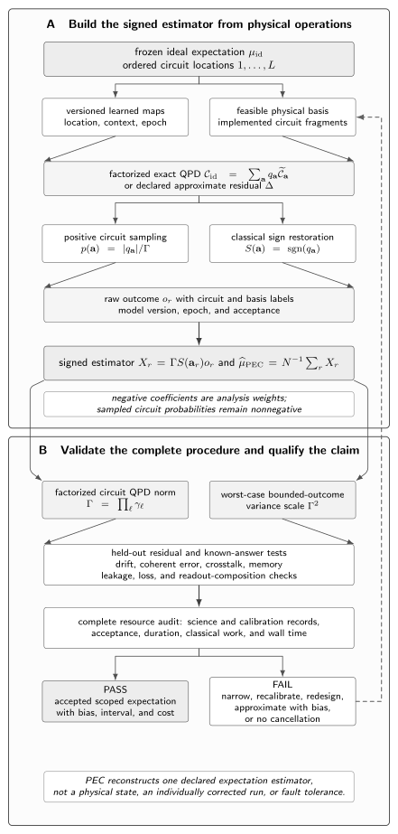
PEC workflow. A versioned noise model and experimentally implementable basis produce a signed decomposition; absolute coefficients define circuit sampling, signs restore the linear combination, and the factorized circuit quasiprobability norm $\Gamma$ sets a worst-case bounded-outcome variance scale $\Gamma^2$. Held-out residual, drift, leakage, and resource audits decide whether the reported observable estimate is accepted, narrowed, recalibrated, redesigned, or not cancelled. The workflow reconstructs an expectation-value estimator, not a physical state or a fault-tolerant computation.

Compose Corrections in Circuit Order

Place corrections on the licensed side

Composition order is observable even in the smallest formal signed-estimator example. Prepare $|+\rangle$, apply an ideal Hadamard, place a bit-flip channel $\mathcal N_{0.1}$ after it, and measure $Z$. The ideal output is $|0\rangle$, so the ideal expectation is one; the noisy expectation is $1-2p=0.8$. Applying the licensed quasiprobability representation of $\mathcal N_{0.1}^{-1}$ after the noisy gate gives signed-estimator expectation one in the exact model.

Moving that inverse before the Hadamard does not work. The input $|+\rangle$ is invariant under bit flips, so the formal inverse leaves it unchanged; the Hadamard then prepares $|0\rangle$, and the later physical bit-flip noise still returns $0.8$. Thus

$$\mathcal N^{-1}\circ\mathcal N\circ\mathcal H \ne \mathcal N\circ\mathcal H\circ\mathcal N^{-1}$$

on the declared input and observable. A compiler that commutes, cancels, or merges sampled corrections must preserve the characterized complete map, not only the ideal gate identity.

Build locationwise circuit samples

For independently sampled labels $a_1,\ldots,a_L$, define

$$p(\boldsymbol a) = \prod_{\ell=1}^{L}p_{\ell a_\ell}, \qquad S(\boldsymbol a) = \prod_{\ell=1}^{L}s_{\ell a_\ell}, \qquad \Gamma = \prod_{\ell=1}^{L}\gamma_\ell.$$

Execute the selected physical maps in the same time order as the circuit and record

$$X=\Gamma S(\boldsymbol a)o.$$

The proof expands the ordered product of linear combinations. It does not commute superoperators as if they were numbers: distributivity supplies a sum over ordered circuit variants, while each term preserves the original composition order. Correlated sampling or a circuit-level QPD uses a different joint law and weight, which should be written directly rather than forced into the product notation.

Compare local and circuit-level decompositions

A local construction is operationally convenient because one can sample each location without enumerating every full circuit. Its factorized norm is $\Gamma=\prod_\ell\gamma_\ell$, which can grow exponentially with the number of corrected locations. A circuit-level construction instead writes

$$\mathcal C_{\mathrm{id}} = \sum_\omega q_\omega \widetilde{\mathcal C}_\omega, \qquad \gamma_{\mathrm{global}} = \sum_\omega|q_\omega|.$$

It can exploit cancellations or structure invisible to separate local fits, so $\gamma_{\mathrm{global}}$ need not equal $\Gamma$. It may also require an intractably large set of circuits or a model that is hard to identify. Report which problem was optimized, the physical operation family it allows, and the classical and experimental work needed to sample it. An improvement in norm is not useful if circuit synthesis or model learning becomes unaffordable.

Mari, Shammah, and Zeng (2021) connect probabilistic cancellation to noise scaling, but the constructions remain distinct. Probabilistic amplification samples a physical ensemble with increased nonnegative noise rates for an extrapolation family; PEC samples a signed representation of an inverse. A shared learned model does not make their estimator identities interchangeable.

Keep readout transformations outside channel algebra

Suppose terminal response correction returns a linear estimate $\widehat m=w^{\mathsf T}\widehat p$ and PEC supplies signed circuit weights. The combined estimator may be written as a larger linear form only after the joint record, calibration dependence, and normalization are specified. If the same readout calibration is reused across all PEC variants, it creates shared uncertainty and covariance. If leakage or acceptance changes across variants, the response model may not transfer at all.

Symmetry conditioning and postselection are often nonlinear because they form ratios of accepted weighted sums. ZNE adds another signed combination across a physical scaling family. State the complete order of these transformations, including which raw records and nuisance estimates are shared. Do not apply a gate-noise inverse, readout inverse, and clipping rule independently and then add their reported error bars as though the procedures commuted.

Audit Negativity, Variance, and Total Cost

Define one-norm and squared overhead

This page reserves $\gamma_\ell$ for a local coefficient one-norm, $\Gamma$ for the factorized circuit quasiprobability norm, and $\Gamma^2$ for the associated worst-case variance scale under unit-bounded outcomes. Other papers may call either norm or its square the “sampling overhead”; always translate the definition before comparing numbers.

For many repeated local corrections, even modest norms are costly. Three bit-flip locations with $p=(0.02,0.05,0.08)$ have

$$\gamma_1=\frac{25}{24}, \qquad \gamma_2=\frac{10}{9}, \qquad \gamma_3=\frac{25}{21},$$

and therefore

$$\Gamma = \frac{3125}{2268} \approx1.37787, \qquad \Gamma^2 = \frac{9765625}{5143824} \approx1.89851.$$

This small fixture is benign; a long circuit can make the product prohibitive. Takagi (2021) formulates optimal resource costs for mitigation, emphasizing that the physical implementability set and desired transformation determine the unavoidable price.

Bound variance for bounded observables

For $|o|\le o_{\max}$, the factorized signed record obeys $|X|\le\Gamma o_{\max}$. Under independent identically distributed sampling,

$$\operatorname{Var}(X) = \Gamma^2\mathbb E[o^2] - \mu_{\mathrm{id}}^2 \le \Gamma^2o_{\max}^2,$$

and

$$\operatorname{Var} (\widehat\mu_{\mathrm{PEC}}) = \frac{\operatorname{Var}(X)}{N}.$$

For the three-location fixture with $o_{\max}=1$, a worst-case standard error at most $0.02$ requires

$$N \ge \left\lceil \frac{\Gamma^2}{0.02^2} \right\rceil =4747.$$

That is a conservative bound, not a prediction of the empirical variance. Use the observed signed records, acquisition dependence, and declared confidence procedure for the reported interval. Qin, Chen, and Li (2023) analyze error statistics and scaling of mitigation formulas; their results reinforce the need to distinguish finite statistical spread from residual systematic bias.

Allocate samples without hiding acceptance loss

When terms are acquired in separate strata, an estimator $\sum_aq_a\widehat\mu_a$ has, under independent strata,

$$\operatorname{Var} \left(\sum_aq_a\widehat\mu_a\right) = \sum_a\frac{q_a^2\sigma_a^2}{N_a}.$$

At fixed equal-duration shots, minimizing this expression gives $N_a\propto|q_a|\sigma_a$. Unequal circuit durations replace a shot budget by a cost budget. Shared calibration, paired randomizations, temporal blocks, and adaptive allocation introduce covariance and require the design actually used in the analysis.

If only a fraction $a$ of issued executions is accepted, collecting $N$ accepted records costs $N/a$ issued executions on average only for a stable independent acceptance process. Basis-dependent acceptance can also change the effective sampling distribution. Retain invalid jobs, leakage flags, losses, and postselection counts by basis term; reweight or model them only under a predeclared estimand.

Report calibration and wall-clock costs

PEC needs more than science shots. Count characterization circuits, model selection and holdout records, compiler variants, twirling, resets, queue time, classical fitting, storage, and every rerun after drift. Compare methods at a matched accepted-answer bias and uncertainty budget. Equal requested shots or equal nominal circuit depth is not a matched resource comparison.

Ledger item	Symbol	Estimate	Units	Statistical contribution	Systematic contribution	Reported decision
Science records	$N_{\mathrm{sci}}$	issued, completed, valid, and accepted counts	executions	signed-record variance and dependence	circuit-family mismatch	acquire, stop, or widen interval
Calibration records	$N_{\mathrm{cal}}$	all model and basis probes	executions	parameter covariance	nonidentifiability and SPAM	reuse only within validated epoch
Tuning and holdout	$N_{\mathrm{tune}},N_{\mathrm{hold}}$	disjoint sets and reuse map	circuits	selection uncertainty	holdout consumption	preserve or replace final holdout
Acceptance and loss	$a$	accepted divided by issued	fraction	effective sample reduction	changed conditional estimand	model, narrow, or reject
Circuit duration and depth	$T,D$	distribution across sampled variants	time and layers	unequal cost per record	context and drift exposure	rebalance or redesign basis
Coefficient one-norm	$\Gamma$	full-precision decomposition value	dimensionless	variance scale $\Gamma^2$	sensitivity to fitted model	accept only within norm budget
Total execution	$C_{\mathrm{tot}}$	quantum, classical, storage, and rerun ledger	wall time and currency	achieved interval at total cost	unresolved bias budget	report matched quality–cost result

The general bounds of Takagi, Endo, Minagawa, and Gu (2022), Takagi, Tajima, and Gu (2023), and Tsubouchi, Sagawa, and Yoshioka (2023) apply to specified protocol, estimator, and noise settings. Quek et al. (2024) establish stronger worst-case limitations for broad mitigation classes and circuit families. They rule out careless scalability claims; they do not imply that every finite shallow PEC experiment is useless.

Learn Noise and Propagate Model Uncertainty

Separate calibration, tuning, and holdout records

Write a learned map as

$$\widehat{\mathcal N}_{\ell,c,e}(\widehat\theta),$$

where $\ell$ is location, $c$ is context, $e$ is epoch, and $\widehat\theta$ is estimated from a named calibration dataset. Record the representation, physicality or structural constraints, optimizer, tolerances, uncertainty, and validity interval. State which preparations, operations, and measurements identify each parameter and which gauge conventions are fixed.

Use calibration data to estimate parameters, tuning data to choose basis, regularization, or model class, and a final holdout to test the frozen complete procedure. Strikis et al. (2021) show how learning-based mitigation can use training circuits, but transfer depends on the relationship between training and science domains. Reusing the final holdout to select a better-looking QPD turns it into tuning data.

Propagate coefficient uncertainty

The fitted parameter affects both $q(\widehat\theta)$ and the sampling law $p(\widehat\theta)$. Conditional science variance therefore does not exhaust uncertainty. With independent calibration and science records, a local delta-method approximation is

$$\operatorname{Var}_{\mathrm{total}} (\widehat\mu) \approx \operatorname{Var}_{\mathrm{sci}} (\widehat\mu\mid\widehat\theta) + g_\theta^{\mathsf T} \Sigma_\theta g_\theta,$$

where

$$g_\theta = \frac{\partial \mathbb E[\widehat\mu\mid\theta]} {\partial\theta}.$$

Shared records, epochs, or adaptive decisions add cross terms. A joint block bootstrap can resample calibration and science blocks and refit the QPD in each replicate. Near a singular map or an active optimization constraint, the coefficient map can be nonsmooth; profile bounds, bootstrap distributions, or set-valued uncertainty are safer than a linearized Gaussian interval.

Audit residual channels on held-out probes

For an exact after-gate convention the formal residual is

$$\mathcal R_\ell = \widehat{\mathcal N}_\ell^{-1} \circ \mathcal N_\ell - \mathcal I.$$

The true $\mathcal N_\ell$ is not known simply because a fit produced a matrix. Probe the composed cancellation on held-out states, observables, circuits, basis-operation mixtures, depths, layouts, and epochs matched to the science workload. Report prediction discrepancies and uncertainty. An empirical domain-specific residual supports that domain, not a uniform norm claim over all inputs and ancillas.

Govia et al. (2025) derive experimentally accessible bounds on systematic mitigation error caused by model violation. Such a bound belongs beside the Monte Carlo interval, not inside it by implication. If only a weaker empirical diagnostic is available, label its coverage and blind directions rather than calling it a worst-case guarantee.

Recalibrate or narrow under drift

Interleave raw baselines and model-sensitive sentinels, randomize or block acquisition order, and record timestamps and calibration transitions. Freeze thresholds for parameter changes, held-out discrepancies, acceptance, and coefficient growth. When a threshold fails, start a new epoch or stop; do not merge incompatible epochs because their weighted means happen to agree.

Available responses differ scientifically: recalibration retains the model class in a new epoch; narrowing restricts the supported circuit or time domain; expanding the basis changes the inverse problem; approximate cancellation accepts explicit bias; redesign changes the acquisition; and no cancellation reports that the current evidence does not license inversion. Preserve failed versions so later readers can distinguish drift from outcome-based selection.

Use Pauli and Sparse Pauli–Lindblad Working Forms

Invert a Pauli-transfer model

For a one-qubit Pauli channel,

$$\mathcal N = \sum_{P\in\{I,X,Y,Z\}} c_P\mathcal P, \qquad \mathcal P(\rho)=P\rho P, \qquad c_P\ge0, \qquad \sum_Pc_P=1.$$

On Pauli operator $Q$, the transfer eigenvalue is

$$\eta_Q = \sum_Pc_P\chi(P,Q),$$

where $\chi(P,Q)=+1$ when $P$ and $Q$ commute and $-1$ when they anticommute. If every $\eta_Q$ is nonzero, the inverse coefficients are the Walsh–Hadamard transform

$$q_P = \frac14 \sum_Q \frac{\chi(P,Q)}{\eta_Q}, \qquad \mathcal N^{-1} = \sum_Pq_P\mathcal P.$$

A small $|\eta_Q|$ makes the coefficients sensitive and expensive; a zero value means the channel erased that operator direction and has no exact inverse. Displaying an arbitrary channel in a Pauli basis does not make it Pauli diagonal. The Pauli-noise owner retains approximation diagnostics and convention checks.

Derive the bit-flip quasiprobability decomposition

For

$$\mathcal N_p = (1-p)\mathcal I+p\mathcal X, \qquad 0\le p<\frac12,$$

use $\mathcal X^2=\mathcal I$ to solve

$$\mathcal N_p^{-1} = \frac{1-p}{1-2p}\mathcal I - \frac{p}{1-2p}\mathcal X, \qquad \gamma = \frac1{1-2p}.$$

At $p=0.1$, the coefficients are $q_I=1.125$ and $q_X=-0.125$; the positive sampling probabilities are $0.9$ and $0.1$. The norm is $1.25$. As $p\to1/2$, the $Z$ and $Y$ contrasts vanish, the coefficients diverge, and the channel loses the information PEC would need to reconstruct. A pseudoinverse can define a projected or regularized estimator, but not exact recovery of the erased direction.

Factor sparse Pauli–Lindblad generators

Suppose a physically constrained model has dimensionless integrated generator strengths $\kappa_k$ for a frozen layer or circuit:

$$\mathcal L(\rho) = \sum_k\kappa_k(P_k\rho P_k-\rho), \qquad \kappa_k\ge0, \qquad \mathcal N=e^{\mathcal L}.$$

Pauli-conjugation superoperators commute even when the underlying Pauli strings anticommute up to phase. For one generator,

$$e^{-\kappa_k(\mathcal P_k-\mathcal I)} = \frac{1+e^{2\kappa_k}}2\mathcal I + \frac{1-e^{2\kappa_k}}2\mathcal P_k.$$

Its second coefficient is negative for $\kappa_k>0$, and its one-norm is $e^{2\kappa_k}$. The exact factorized model gives

$$\Gamma = \exp\left(2\sum_k\kappa_k\right), \qquad \Gamma^2 = \exp\left(4\sum_k\kappa_k\right).$$

State whether the sum covers one layer, every repeated layer, or the complete circuit. A fitted negative integrated strength does not license this probability model; revisit constraints or the assumed generator family.

Preserve correlated terms when evidence requires them

van den Berg et al. (2023) demonstrate PEC using sparse Pauli–Lindblad models on noisy processors. Sparse need not mean independent or single-qubit: a multi-qubit Pauli string can represent an evidence-supported correlated component. Deleting it to make the decomposition cheaper can reduce $\Gamma^2$ while increasing systematic bias.

Report candidate supports, selection criteria, parameter uncertainty, held-out predictive gain, and the overhead contribution of retained correlated terms. Noise tailoring used to make the model Pauli-like is part of the frozen physical baseline and resource ledger. It must be repeated or validated in the science circuits rather than treated as a mathematical coordinate change.

Diagnose Coherent, Correlated, Memory, and Leakage Failures

Coherent error exceeds a Pauli-only model

Coherent noise does not make PEC impossible by definition. A sufficiently rich implemented basis and accurate model can represent a unitary overrotation or another coherent component. The failure occurs when a Pauli-only, twirled, or stochastic model is used outside the domain in which it predicts the complete sampled procedure. Coherent residuals can accumulate with circuit structure rather than average like independent faults.

Compare phase-sensitive and Pauli-sensitive holdouts, reverse or vary gate sequences, and test observables that expose off-diagonal transfer components. If physical twirling is used, freeze its ensemble, randomness, compiler action, and cost. A good average fidelity or Pauli error rate does not establish that the omitted coherent direction is harmless for the science observable.

Crosstalk defeats local factorization

A product model assumes that a location’s implemented map is stable under the activity represented elsewhere in the circuit. Crosstalk breaks that premise when simultaneous or neighboring operations change its channel. A product of individually accurate QPDs can then be inaccurate for the joint layer.

Use simultaneous-versus-isolated probes, spectator observables, direction and frequency sweeps, and held-out layer patterns. If evidence supports a cluster map, include a joint basis and pay its identification and one-norm costs. If the required cluster is too large to learn or sample, narrow concurrency or decline cancellation. A local residual measured in isolation is not evidence for a global factorization.

Memory invalidates a fixed location channel

When later noise depends on earlier controls, environment state, resets, or outcomes, one fixed map per location may not describe the experiment. A PEC sample changes the sequence of basis operations and can therefore change the future environment history it was meant to cancel. The algebra of independent one-step channels then omits the relevant conditional dynamics.

Interleave history variants, causal breaks, repeated baselines, and temporal blocks. The Markovian and Non-Markovian Noise page owns the distinction among fixed-step composition, interval products, CP-divisibility, witnesses, and multitime escalation. A context-augmented PEC model is acceptable only if those extra dependencies are identifiable and validated; otherwise report the memory boundary rather than claiming an unbiased inverse.

Leakage and loss change the state space

Leakage moves population outside the modeled computational subspace; loss or invalid acquisition can make the retained branch trace decreasing. A trace-preserving Pauli inverse on the retained subspace cannot reconstruct unobserved population or silently normalize it away. Return dynamics can also carry phase and history information that a scalar survival correction misses.

The Leakage and Crosstalk owner supplies full-space, retained-branch, leakage, seepage, and coherent- return models. PEC must either use that enlarged state and outcome space or state a conditional estimand with explicit survival and acceptance costs. Record leakage flags and lost executions by sampled basis choice, because basis-dependent loss distorts both the target and the nominal sampling law.

Validate Composed Procedures and Apply Stop Rules

Test identities on matched validation workloads

Validation should exercise the complete pipeline: model fit, QPD construction, physical circuit substitution, sampling, readout treatment, acceptance, weighting, and uncertainty. Use identity and known-answer circuits, Clifford or otherwise tractable surrogates, randomized and structured holdouts, null cases, depth sweeps, layouts, epochs, and basis mixtures matched to the science workload. Reserve some high-weight and rare basis choices rather than validating only the most probable branch.

An ideal simulator can verify the target-preserving algebra and circuit order; it cannot validate the physical noise model. Hardware holdouts test transfer but may have only partial references. Combine complementary tests and state their blind directions. Device Characterization owns diagnostic experimental design; this page owns whether the evidence licenses the signed inverse used in the estimator.

Compare raw, mitigated, and reference predictions

Report raw and PEC estimates with their joint uncertainty, trusted reference or validation prediction, residual, accepted bias budget, and total cost. Repeat raw baselines across the PEC acquisition so drift is visible. A favorable PEC shift is not evidence if the reference was used to tune the model, basis, regularization, or stopping time.

Use more than final-answer agreement. Check per-circuit residuals, calibration predictions, basis-conditioned outcomes, signed-record distribution, coefficient stability, acceptance, and epoch dependence. A PEC result can agree with a classical value while the model fails elsewhere, or disagree because the classical reference, compiler mapping, observable convention, or measurement model is wrong. Preserve those alternatives in the conclusion.

Accept, narrow, redesign, or do not cancel

Apply the predeclared thresholds before inspecting whether the final value is desirable. Exact PEC is rejected when the target is outside the feasible span, a needed transfer direction is singular, coefficient uncertainty or $\Gamma^2$ exceeds budget, held-out residual exceeds the bias allowance, drift breaks the epoch, acceptance collapses, or unmodeled leakage, memory, or crosstalk controls the result. Approximate-with-bias, narrow-domain, recalibrate, redesign-basis, and no-cancel are distinct outcomes.

Failure mode	Observable symptom	Algebraic cause	Required diagnostic	Invalid shortcut	Permitted response	Remaining claim	Canonical owner
Incomplete basis	irreducible held-out residual	target outside real span of feasible maps	rank, residual, and new-basis holdouts	use unconstrained ideal maps	expand basis, approximate with bias, or stop	scoped residual bound only	Quantum Channels for QI
Near-singular map	unstable or enormous coefficients	small transfer singular value	spectrum and perturbation analysis	call a pseudoinverse exact	narrow target, regularize with bias, or stop	projected estimator if declared	Lower Bounds and Limitations
Model drift	epoch-dependent residual or norm	learned map no longer matches execution	interleaved sentinels and blocked analysis	pool epochs for a nicer mean	recalibrate or narrow time window	epoch-scoped result	Device Characterization
Coherent residual	sequence-sensitive oscillation	Pauli-only model omits phase action	phase-sensitive reversed sequences	infer adequacy from average fidelity	enrich or physically tailor model	only tested sequence family	Pauli Noise and Depolarizing Channels
Crosstalk	simultaneous and isolated predictions differ	local maps do not factor	spectator and joint-layer probes	multiply isolated QPDs	cluster model, schedule change, or stop	validated concurrency domain	Leakage and Crosstalk
Memory	outcome depends on prior sampled choices	no fixed one-step channel	history variants and causal breaks	relabel time dependence as shot noise	context model, reset redesign, or stop	supported history class	Markovian and Non-Markovian Noise
Leakage or loss	basis-dependent survival and normalization	modeled subspace is not closed	full-space flags and return tests	renormalize retained records silently	augment state space or declare conditioning	conditional or full-space target	Leakage and Crosstalk
Readout composition	correction order changes estimate	estimator maps or nuisance records are shared	end-to-end replay and covariance	add independent error bars	joint estimator or separate acquisition	declared composed estimator	Measurement Error Mitigation
Excessive overhead	uncertainty or runtime misses budget	signed norm compounds with depth	total-resource and achieved-error ledger	quote $\Gamma$ as actual shots	reduce scope, redesign QPD, or stop	finite budget comparison	Reporting Standards

Three Reproducible PEC Audits

Audit 1 — Bit-flip signed sampling

Take $p=0.1$ and an ideal $Z$ expectation $0.6$, with $\pm1$ measurement outcomes. The bit-flip channel attenuates it to $0.48$. The inverse coefficients $1.125$ and $-0.125$ give norm $1.25$ and sampling probabilities $0.9$ and $0.1$. The identity branch has mean $0.48$; the physical $X$ branch has mean $-0.48$, and its negative analysis sign reverses it. Their weighted expectation is therefore $0.6$.

For binary outcomes, every signed record has squared magnitude $1.25^2$, so the per-shot PEC variance is $1.25^2-0.6^2=1.2025$. At $N=10000$ the standard error is about $0.01097$. The raw estimator has smaller variance but bias $-0.12$; its mean-squared error is $0.01447696$, compared with $0.00012025$ for the exact-model PEC fixture. This equal-$N$ comparison excludes calibration and acceptance costs; it is not a matched total-resource claim, and it changes under model error.

Audit 2 — Circuit order and composed overhead

The $|+\rangle$–Hadamard example gives ideal expectation one, noisy expectation $0.8$, after-noise formal signed-estimator expectation one, and incorrectly moved pre-Hadamard formal signed-estimator expectation $0.8$. It detects a placement bug that coefficient normalization alone cannot find.

For $p=(0.02,0.05,0.08)$, the local norms are $25/24$, $10/9$, and $25/21$. Their product is $3125/2268$, its square is $9765625/5143824$, and the unit-bounded worst-case requirement for standard error at most $0.02$ is $4747$ records. This is the algebraic cost fixture, not a claim that three physical locations are independent or exactly bit-flip.

Audit 3 — Model mismatch and singularity

Let the true bit-flip rate be $0.1$ while the learned rate is $0.08$. Applying the learned inverse to raw mean $0.48$ returns

$$\frac{0.48}{1-2(0.08)} = \frac47,$$

so the bias relative to $0.6$ is $-1/35\approx-0.02857$. Here $1/35$ is an observable- and domain-specific held-out discrepancy, not a uniform channel norm. A frozen absolute-bias budget $0.02$ rejects the result even if its Monte Carlo interval is tiny. At $p=0.5$, the contrast is exactly zero and no exact inverse exists. The finite audits below reconstruct all three cases.

const tolerance = 1e-12;

function assertClose(actual, expected, label, scale = 1) {
  if (Math.abs(actual - expected) > tolerance * Math.max(scale, 1)) {
    throw new Error(`${label}: expected ${expected}, received ${actual}`);
  }
}

function assertTrue(condition, label) {
  if (!condition) throw new Error(label);
}

function bitFlipQpd(p) {
  const contrast = 1 - 2 * p;
  assertTrue(Math.abs(contrast) > tolerance, 'bit-flip channel is singular');
  const qI = (1 - p) / contrast;
  const qX = -p / contrast;
  const gamma = Math.abs(qI) + Math.abs(qX);
  return { contrast, qI, qX, gamma, pI: Math.abs(qI) / gamma, pX: Math.abs(qX) / gamma };
}

const ideal = 0.6;
const trueRate = 0.1;
const shots = 10000;
const qpd = bitFlipQpd(trueRate);
const rawMean = ideal * qpd.contrast;
const xBranchMean = -rawMean;
const pecMean = qpd.gamma * (qpd.pI * rawMean + qpd.pX * (-1) * xBranchMean);
const pecPerShotVariance = qpd.gamma ** 2 - pecMean ** 2;
const pecSE = Math.sqrt(pecPerShotVariance / shots);
const rawMSE = (rawMean - ideal) ** 2 + (1 - rawMean ** 2) / shots;
const pecMSE = pecPerShotVariance / shots;

assertClose(qpd.qI, 1.125, 'qI');
assertClose(qpd.qX, -0.125, 'qX');
assertClose(qpd.gamma, 1.25, 'gamma');
assertClose(qpd.pI, 0.9, 'pI');
assertClose(qpd.pX, 0.1, 'pX');
assertClose(rawMean, 0.48, 'raw mean');
assertClose(pecMean, 0.6, 'PEC mean');
assertClose(pecPerShotVariance, 1.2025, 'PEC per-shot variance');
assertClose(pecSE, 0.010965856099730654, 'PEC standard error');
assertClose(rawMSE, 0.01447696, 'raw MSE');
assertClose(pecMSE, 0.00012025, 'PEC MSE');

const hadamardIdeal = 1;
const noisyAfterHadamard = 1 - 2 * trueRate;
const correctedAfter = noisyAfterHadamard / (1 - 2 * trueRate);
const incorrectlyMovedBefore = noisyAfterHadamard;
assertClose(hadamardIdeal, 1, 'Hadamard ideal');
assertClose(noisyAfterHadamard, 0.8, 'Hadamard noisy');
assertClose(correctedAfter, 1, 'after-noise inverse');
assertClose(incorrectlyMovedBefore, 0.8, 'moved inverse');

const localRates = [0.02, 0.05, 0.08];
const localGammas = localRates.map((p) => bitFlipQpd(p).gamma);
const Gamma = localGammas.reduce((product, value) => product * value, 1);
const GammaSquared = Gamma ** 2;
const requiredShots = Math.ceil(GammaSquared / 0.02 ** 2);
assertClose(localGammas[0], 25 / 24, 'first local gamma');
assertClose(localGammas[1], 10 / 9, 'second local gamma');
assertClose(localGammas[2], 25 / 21, 'third local gamma');
assertClose(Gamma, 3125 / 2268, 'Gamma');
assertClose(GammaSquared, 9765625 / 5143824, 'Gamma squared');
assertTrue(requiredShots === 4747, 'worst-case shot ceiling');

const learnedRate = 0.08;
const learnedMitigatedMean = rawMean / (1 - 2 * learnedRate);
const learnedBias = learnedMitigatedMean - ideal;
const heldOutAbsoluteResidual = Math.abs(learnedBias);
const acceptedBiasBudget = 0.02;
const decision = heldOutAbsoluteResidual > acceptedBiasBudget ? 'REJECT' : 'ACCEPT';
assertClose(learnedMitigatedMean, 4 / 7, 'learned mitigated mean');
assertClose(learnedBias, -1 / 35, 'learned bias');
assertClose(heldOutAbsoluteResidual, 1 / 35, 'held-out residual');
assertTrue(decision === 'REJECT', 'model-mismatch decision');
assertTrue(1 - 2 * 0.5 === 0, 'singular boundary');

console.log('Probabilistic-error-cancellation finite audits: PASS');

These arithmetic tests verify signs, normalization, circuit order, product overhead, finite variance, a frozen stop rule, and the singular boundary. They do not validate a hardware channel, a Pauli approximation, an independence assumption, or workload transfer. Those remain empirical obligations.

Canonical Owners and Common Claim Failures

Canonical handoffs

Use the Error Mitigation Overview to choose among mitigation families and Zero-Noise Extrapolation for target-preserving physical noise scaling and intercept inference. Use VQE and Digital Quantum Simulation for algorithm-specific objective, mapping, synthesis, and interpretation. Reporting Standards owns durable raw-data and provenance artifacts, while Lower Bounds and Limitations owns formal asymptotic assumptions and resource regimes.

Verification of Quantum Advantage retains correctness, hardness, and classical-frontier claims. Why Quantum Error Correction Is Possible owns encoded recovery and logical protection. Cai et al. (2023) provide a broad review of mitigation families, but no overview transfers a specialist license from one estimator to another.

Common claim failures

An abstract basis is called executable. Replace every ideal basis symbol by the characterized physical circuit fragment that is actually sampled, or reject the decomposition.

Conditional unbiasedness is called observed fact. State the exact model, span, placement, context, acquisition, and normalization conditions; report finite model uncertainty and held-out residual separately.

The norm is called the shot count. Define $\Gamma$ and $\Gamma^2$, then report empirical signed-record variance, acceptance, dependence, and total cost at the requested error budget.

A Pauli model is treated as universal. Test coherent, correlated, memory, leakage, and loss alternatives. Retain correlated terms supported by evidence, even when they increase cost.

A favorable value is clipped into range. Preserve the signed estimate and diagnose variance or mismatch. A constrained estimator must be predeclared and validated as a different procedure.

A finite mitigated observable is called protection. PEC reconstructs a selected expectation under assumptions; it neither repairs the physical state nor supplies fault-tolerant depth.

Exercises

Derive the bit-flip inverse. Starting from $\mathcal N_p=(1-p)\mathcal I+p\mathcal X$, solve for the two inverse coefficients, their signs, sampling probabilities, and one-norm; identify the invertibility boundary and interpret its approach.

Solution

Write the inverse as $a\mathcal I+b\mathcal X$ and use $\mathcal X^2=\mathcal I$. Matching identity and $\mathcal X$ coefficients gives $a=(1-p)/(1-2p)$ and $b=-p/(1-2p)$. For $p<1/2$, their sampling probabilities are $1-p$ and $p$, and $\gamma=1/(1-2p)$. At $p=1/2$ the contrast vanishes; approaching it makes the inverse coefficients and variance cost diverge because the channel erases an operator direction.

Prove conditional unbiasedness. Starting from a finite implemented-map decomposition, derive the absolute-coefficient sampling estimator and list every condition used by the expectation identity.

Solution

For $\mathcal C_{\mathrm{id}}=\sum_aq_a\widetilde{\mathcal C}_a$, set $\gamma=\sum_a|q_a|$, sample $a$ with $|q_a|/\gamma$, and record $X=\gamma\operatorname{sgn}(q_a)o$. Summing conditional expectations returns $\sum_aq_a\operatorname{Tr}[O\widetilde{\mathcal C}_a(\rho)]$. Equality to the ideal target requires exact implemented maps, exact target equality, the declared circuit order and context, correct sampling, stable outcome normalization, and no unmodeled acceptance or drift.

Audit correction placement. Use the $|+\rangle$, Hadamard, bit-flip, and terminal-$Z$ example to calculate after-gate and incorrectly moved before-gate inverse results and explain the noncommuting failure.

Solution

The Hadamard maps $|+\rangle$ to $|0\rangle$, whose ideal $Z$ expectation is one. A bit-flip channel with rate $p$ reduces it to $1-2p$; its inverse applied afterward restores one. Applied before the Hadamard, the inverse acts trivially on $|+\rangle$, because that state is invariant under $X$. The later noise still returns $1-2p$. The two placements differ because the gate and inverse channel are not freely commutable.

Compose the overhead. For $p=(0.02,0.05,0.08)$, compute all local norms, $\Gamma$, $\Gamma^2$, and the worst-case shots required for standard error at most $0.02$; distinguish the bound from an empirical requirement.

Solution

The local norms $1/(1-2p)$ are $25/24$, $10/9$, and $25/21$. Their product is $\Gamma=3125/2268\approx1.37787$, and $\Gamma^2=9765625/5143824\approx1.89851$. Unit-bounded outcomes therefore give $N\ge\lceil\Gamma^2/0.02^2\rceil=4747$. This uses a worst-case second-moment bound and independent records, not a fitted requirement. The actual requirement uses the measured signed-record variance, dependence, acceptance, and desired confidence procedure.

Bound an approximate decomposition. Given a residual superoperator and observable norm, derive a state-specific trace-norm bound and a uniform diamond-norm bound, then state what validation would support the narrower claim.

Solution

If the decomposition residual is $\Delta$, Hölder duality gives $|\operatorname{Tr}[O\Delta(\rho)]|\le \lVert O\rVert_\infty\lVert\Delta(\rho)\rVert_1$. Maximizing the induced trace norm over inputs and an ancilla gives the uniform bound $\lVert O\rVert_\infty\lVert\Delta\rVert_\diamond$. A narrower claim needs held-out states, observables, circuit structures, and contexts representative of the stated science domain, with selection kept separate from final evaluation.

Propagate a learned-rate error. With true $p=0.1$ and learned $\widehat p=0.08$, compute the PEC bias for ideal expectation $0.6$, compare it with a $0.02$ bias budget, and choose an explicit decision.

Solution

The true channel returns raw mean $0.6(1-0.2)=0.48$. The learned inverse rescales by $1/(1-0.16)=25/21$, producing $4/7$. Its bias is $4/7-3/5=-1/35\approx-0.02857$. The absolute residual exceeds the frozen $0.02$ budget, so the decision is REJECT for exact PEC. One may recalibrate, narrow the epoch, or report a separately licensed approximate result, but a small Monte Carlo interval cannot reverse the failed bias test.

Factor a sparse Pauli–Lindblad inverse. Derive the two coefficients and one-norm for one generator, extend them to several Pauli strings, and explain why deleting an evidence-supported correlated term can bias PEC.

Solution

For dimensionless integrated strength $\kappa$ in generator $\kappa(\mathcal P-\mathcal I)$, use $\mathcal P^2=\mathcal I$ to obtain inverse coefficients $(1+e^{2\kappa})/2$ and $(1-e^{2\kappa})/2$. Their one-norm is $e^{2\kappa}$. Commuting Pauli-conjugation superoperators multiply, yielding $\Gamma=e^{2\sum_k\kappa_k}$. Omitting a correlated $P_k$ replaces the learned channel by a different model; the cheaper norm then accompanies a residual action and possible systematic observable bias.

Write a no-cancel record. Given a near-singular transfer eigenvalue, falling acceptance, and a failed held-out residual, complete the resource and failure ledgers and write a scoped negative conclusion without claiming hardware-wide impossibility.

Solution

Record the small eigenvalue and coefficient sensitivity, $\Gamma$ and $\Gamma^2$, issued and accepted counts, acceptance by basis choice, calibration and holdout sizes, residual with uncertainty, epoch, and total runtime. The conclusion is: “For this circuit, observable, basis, model version, and epoch, exact PEC is not licensed within the stated bias and resource budgets.” This does not rule out a redesigned basis, narrower target, new calibration, other device context, or error-corrected architecture.

References

• Z. Cai, R. Babbush, S. C. Benjamin, S. Endo, W. J. Huggins, Y. Li, J. R. McClean, and T. E. O’Brien, “Quantum Error Mitigation,” Reviews of Modern Physics 95, 045005 (2023), doi:10.1103/RevModPhys.95.045005.

• S. Endo, S. C. Benjamin, and Y. Li, “Practical Quantum Error Mitigation for Near-Future Applications,” Physical Review X 8, 031027 (2018), doi:10.1103/PhysRevX.8.031027.

• L. C. G. Govia, S. Majumder, S. V. Barron, B. Mitchell, A. Seif, Y. Kim, C. J. Wood, E. J. Pritchett, S. T. Merkel, and D. C. McKay, “Bounding the Systematic Error in Quantum Error Mitigation due to Model Violation,” PRX Quantum 6, 010354 (2025), doi:10.1103/PRXQuantum.6.010354.

• A. Mari, N. Shammah, and W. J. Zeng, “Extending Quantum Probabilistic Error Cancellation by Noise Scaling,” Physical Review A 104, 052607 (2021), doi:10.1103/PhysRevA.104.052607.

• C. Piveteau, D. Sutter, and S. Woerner, “Quasiprobability Decompositions with Reduced Sampling Overhead,” npj Quantum Information 8, 12 (2022), doi:10.1038/s41534-022-00517-3.

• D. Qin, Y. Chen, and Y. Li, “Error Statistics and Scalability of Quantum Error Mitigation Formulas,” npj Quantum Information 9, 35 (2023), doi:10.1038/s41534-023-00707-7.

• Y. Quek, D. Stilck França, S. Khatri, J. J. Meyer, and J. Eisert, “Exponentially Tighter Bounds on Limitations of Quantum Error Mitigation,” Nature Physics 20, 1648–1658 (2024), doi:10.1038/s41567-024-02536-7.

• C. Song, J. Cui, H. Wang, J. Hao, H. Feng, and Y. Li, “Quantum Computation with Universal Error Mitigation on a Superconducting Quantum Processor,” Science Advances 5, eaaw5686 (2019), doi:10.1126/sciadv.aaw5686.

• A. Strikis, D. Qin, Y. Chen, S. C. Benjamin, and Y. Li, “Learning-Based Quantum Error Mitigation,” PRX Quantum 2, 040330 (2021), doi:10.1103/PRXQuantum.2.040330.

• R. Takagi, “Optimal Resource Cost for Error Mitigation,” Physical Review Research 3, 033178 (2021), doi:10.1103/PhysRevResearch.3.033178.

• R. Takagi, S. Endo, S. Minagawa, and M. Gu, “Fundamental Limits of Quantum Error Mitigation,” npj Quantum Information 8, 114 (2022), doi:10.1038/s41534-022-00618-z.

• R. Takagi, H. Tajima, and M. Gu, “Universal Sampling Lower Bounds for Quantum Error Mitigation,” Physical Review Letters 131, 210602 (2023), doi:10.1103/PhysRevLett.131.210602.

• K. Temme, S. Bravyi, and J. M. Gambetta, “Error Mitigation for Short-Depth Quantum Circuits,” Physical Review Letters 119, 180509 (2017), doi:10.1103/PhysRevLett.119.180509.

• K. Tsubouchi, T. Sagawa, and N. Yoshioka, “Universal Cost Bound of Quantum Error Mitigation Based on Quantum Estimation Theory,” Physical Review Letters 131, 210601 (2023), doi:10.1103/PhysRevLett.131.210601.

• E. van den Berg, Z. K. Minev, A. Kandala, and K. Temme, “Probabilistic Error Cancellation with Sparse Pauli–Lindblad Models on Noisy Quantum Processors,” Nature Physics 19, 1116–1121 (2023), doi:10.1038/s41567-023-02042-2.

• S. Zhang, Y. Lu, K. Zhang, W. Chen, Y. Li, J.-N. Zhang, and K. Kim, “Error-Mitigated Quantum Gates Exceeding Physical Fidelities in a Trapped-Ion System,” Nature Communications 11, 587 (2020), doi:10.1038/s41467-020-14376-z.