VQE

Short Definition

The variational quantum eigensolver (VQE) estimates the lowest eigenvalue of a specified Hermitian operator $H$ by minimizing its expectation value over a parameterized family of quantum states:

$$E(\boldsymbol{\theta}) = \langle \psi(\boldsymbol{\theta}) \rvert H \lvert \psi(\boldsymbol{\theta}) \rangle.$$

If $E_0$ is the exact ground-state energy of $H$, the Rayleigh–Ritz principle gives

$$E(\boldsymbol{\theta}) \geq E_0$$

for every normalized trial state. A quantum processor prepares the trial state and estimates terms in $H$; a classical optimizer chooses new parameters. VQE trades the long coherent evolution used by phase estimation for many shorter state preparations, measurements, and adaptive quantum–classical round trips.

This page is the canonical home for that ground-energy contract, the variational bound, Hamiltonian averaging, VQE ansatzes, energy-specific error budgets, excited-state extensions, validation, and complete resource accounting. Variational Quantum Algorithms owns the general hybrid loop, parameter-shift calculus, quantum natural gradient, barren plateaus, and optimizer families. Hybrid Quantum Simulation owns projected time evolution and quantum embedding, which may use VQE as a state or impurity solver but have additional interface and feedback errors. Electronic-structure pages own the physical approximations used to construct molecular Hamiltonians. Simulation of Quantum Chemistry owns the complete handoff from a declared molecular model through active-space and fermion-to-qubit encoding to VQE, phase estimation, dynamics, resources, and a chemically interpreted output. Quantum Algorithms for Chemistry and Materials compares VQE and adaptive variants with phase-estimation and dynamics routes for a fixed chemistry or materials task; this page retains the VQE guarantee, estimator, ansatz, optimization, and validation contract.

Problem Contract

An ideal VQE instance specifies:

1. a finite-dimensional Hermitian operator $H$;
2. a state-preparation reference $\lvert\psi_{\mathrm{ref}}\rangle$;
3. an implementable normalized family $\lvert\psi(\boldsymbol{\theta})\rangle$;
4. a measurement protocol for $E(\boldsymbol{\theta})$ and any constraints;
5. an optimizer, initialization, stopping rule, and total budget;
6. a validation procedure for the selected parameters.

The primary output may be an energy estimate, a circuit preparing an approximate ground state, or both. These outputs have different success criteria. A precise energy does not automatically imply high state fidelity when the spectral gap is small, and a useful prepared state may support observables whose accuracy is not captured by the energy alone.

The input model matters. If $H$ is supplied as a list of Pauli coefficients, the cost of deriving those coefficients has been placed outside the VQE boundary. If molecular integrals, orbital optimization, active-space selection, or qubit reduction are performed as part of the workflow, their classical cost and approximation error belong in the report.

The Quantum Algorithms and Complexity chapter guide keeps the physical problem and encoded model, algorithmic procedure, selected validation record, resource boundary, and comparison claim distinct.

Rayleigh–Ritz Guarantee

Let

$$H = \sum_{k=0}^{d-1} E_k \lvert E_k\rangle\langle E_k\rvert, \qquad E_0\leq E_1\leq\cdots.$$

Expand a normalized trial state as

$$\lvert\psi\rangle = \sum_k c_k\lvert E_k\rangle, \qquad \sum_k\lvert c_k\rvert^2=1.$$

Then

$$\begin{aligned} \langle H\rangle_\psi &= \sum_k \lvert c_k\rvert^2E_k \\ &= E_0 + \sum_{k>0} \lvert c_k\rvert^2 \left( E_k-E_0 \right) \\ &\geq E_0. \end{aligned}$$

The proof uses only Hermiticity, normalization, and the ordering of the spectrum. It is independent of how the state is prepared.

Restricted-family minimum

VQE searches only its ansatz family. Define

$$E_\Theta = \inf_{\boldsymbol{\theta}\in\Theta} E(\boldsymbol{\theta}).$$

The exact relation is

$$E_\Theta \geq E_0.$$

Equality requires the family to contain a ground state, or to approach one in the relevant closure. An optimizer can converge perfectly and still return a poor answer when $E_\Theta-E_0$ is large. This representation error is distinct from failure to locate the best state already available in the family.

What the upper bound applies to

The bound concerns the exact expectation of the same operator $H$ on a valid normalized state. It does not automatically apply to:

• a finite-shot sample mean on one realization;
• an expectation of an implemented operator $H_{\mathrm{impl}}\neq H$;
• a readout-biased estimator;
• an extrapolated or quasiprobability-mitigated estimate;
• a Hamiltonian produced by an unintended mapping or tapering sector;
• the exact energy of the physical molecule rather than the supplied finite-basis model.

A reported value below a trusted $E_0$ is therefore a diagnostic. It can arise from statistics, calibration, observable mismatch, mitigation, selection, or analysis. It is not evidence of a state with energy below the ground state.

Mixed states still obey the bound

State-preparation noise produces a density operator $\rho$ when the evolution is a physical trace-preserving process. If the intended $H$ is measured exactly,

$$\operatorname{Tr}(\rho H) = \sum_k E_k \langle E_k\rvert\rho\lvert E_k\rangle \geq E_0.$$

Thus decoherence does not repeal the variational principle. It usually redistributes weight toward excited states and degrades accuracy. The bound is lost at the estimator level when the measured observable, calibration model, or postprocessing no longer corresponds to an exact expectation of $H$ on a physical state.

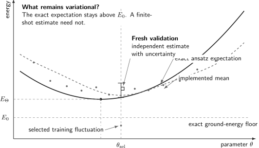
The exact ansatz energy remains above $E_0$, and its minimum $E_\Theta$ can remain higher because the family is restricted. The implemented objective may be distorted, while finite-shot training estimates can fluctuate below either curve or even below $E_0$. Fresh validation estimates the selected workflow output; it does not retroactively turn noisy training samples into variational bounds.

Energy Error and State Fidelity

Assume a nondegenerate ground state and gap

$$\Delta = E_1-E_0 > 0.$$

The spectral expansion gives

$$E-E_0 \geq \Delta \left( 1-\lvert c_0\rvert^2 \right).$$

Therefore

$$\lvert \langle E_0\vert\psi\rangle \rvert^2 \geq 1- \frac{E-E_0}{\Delta}.$$

A small energy error certifies high ground-state overlap only relative to a known gap. When $\Delta$ is small, a visibly accurate energy may coexist with substantial excited-state weight. In a degenerate ground space, replace $\lvert c_0\rvert^2$ by the total weight in that space and use the gap above it.

This bound also requires knowledge of $E_0$, which is the quantity VQE seeks. A rigorous lower bound $L\leq E_0$ can be combined with an upper estimate $U\geq E_0$ to form an interval. Then

$$1-F_0 \leq \frac{U-L}{\Delta}$$

under the same gap assumptions. Producing practical lower bounds is a separate certification problem; dual variational methods are one active direction.

Energy variance

The energy variance is

$$\sigma_H^2 = \langle H^2\rangle - \langle H\rangle^2.$$

It vanishes exactly when the state has support inside one eigenspace. A small variance indicates concentration near one or more nearby eigenvalues, but does not by itself identify the ground state. Measuring $H^2$ can also be expensive: the product of two Pauli sums may contain many terms even after algebraic simplification.

A Four-Part VQE Error Budget

Let

$$\boldsymbol{\theta}_* \in \operatorname*{arg\,min}_{\boldsymbol{\theta}\in\Theta} E(\boldsymbol{\theta}),$$

and let $\widehat{\boldsymbol{\theta}}$ be the selected output. Denote the implemented hardware estimand by $E_{\mathrm{phys}}(\widehat{\boldsymbol{\theta}})$ and its finite-data estimate by $\widehat E$. Then

$$\begin{aligned} \widehat E-E_0 &= \left( \widehat E-E_{\mathrm{phys}} \right) \\ &\quad+ \left( E_{\mathrm{phys}} - E(\widehat{\boldsymbol{\theta}}) \right) \\ &\quad+ \left( E(\widehat{\boldsymbol{\theta}}) - E(\boldsymbol{\theta}_*) \right) \\ &\quad+ \left( E(\boldsymbol{\theta}_*)-E_0 \right). \end{aligned}$$

The terms are:

1. statistical and analysis error in the reported estimator;
2. implementation error from noise, drift, readout, compilation, and observable mismatch;
3. optimization error within the chosen family;
4. representation error of the family itself.

For chemistry, a fifth layer sits outside this equation: model error between $E_0$ of the encoded Hamiltonian and the desired physical quantity. Basis truncation, active spaces, frozen cores, relativistic effects, Born–Oppenheimer separation, and geometry all contribute.

These terms need not have fixed signs. The ideal optimization and representation terms are nonnegative. Statistical fluctuations, mitigation, and model differences can be positive or negative.

From a Physical Problem to a Qubit Hamiltonian

VQE solves the operator it is given. For a molecular calculation at fixed nuclear geometry, a common second-quantized electronic Hamiltonian is

$$\begin{aligned} H_{\mathrm e} &= E_{\mathrm{nn}} + \sum_{p,q} h_{pq} a_p^\dagger a_q \\ &\quad+ \frac12 \sum_{p,q,r,s} h_{pqrs} a_p^\dagger a_q^\dagger a_s a_r. \end{aligned}$$

Here the one- and two-electron integrals depend on the orbital basis and nuclear geometry, while $E_{\mathrm{nn}}$ is the nuclear repulsion energy. The canonical many-particle operator construction is developed in Many-Particle Hamiltonians; Electronic Structure Overview owns the physical and chemical approximation hierarchy.

A fermion-to-qubit transformation produces

$$H_{\mathrm q} = \sum_{j=0}^{M-1} h_j P_j,$$

where each $P_j$ is an $n$-qubit Pauli word. Jordan–Wigner, parity, and Bravyi–Kitaev-type encodings differ in locality, symmetry exposure, and compilation cost. Qubit tapering can remove fixed symmetry sectors. These transformations must preserve the intended spectrum within the selected sector; a smaller qubit count is not useful if the wrong charge, spin, or parity sector is retained.

The full model record includes:

• geometry, units, nuclear charges, and external fields;
• orbital basis and integral-generation software;
• charge, multiplicity, and symmetry sector;
• frozen-core and active-space choices;
• integral thresholds and coefficient precision;
• fermion-to-qubit map, qubit order, and phase conventions;
• tapering symmetries and selected eigenvalues;
• constant energy shifts.

For spin and lattice models, the Hamiltonian may already be a sum of local Pauli operators. The VQE contract is unchanged; only the model-construction layer differs.

Choosing the Trial Family

The ansatz must balance reachability, circuit cost, symmetry, and trainability. No family is uniformly best.

Reference states

For weakly correlated molecular regimes, the Hartree–Fock determinant is a common reference. It is easy to prepare in an occupation encoding and fixes particle number. Near bond dissociation, transition-metal complexes, or other strongly correlated regimes, a single determinant can have poor overlap with the target. Multireference, active-space, tensor-network, or classically preoptimized references may then be more appropriate.

A strong classical reference is not an unfair shortcut. It is part of the hybrid algorithm and must be included in the cost and comparator. If the classical procedure already returns the desired energy and observables, the incremental role of the quantum step must be stated.

Unitary coupled cluster

For occupied orbitals $i,j$ and virtual orbitals $a,b$, define

$$T = T_1+T_2+\cdots,$$

with

$$T_1 = \sum_{i,a} t_i^a a_a^\dagger a_i,$$

and

$$T_2 = \frac14 \sum_{i,j,a,b} t_{ij}^{ab} a_a^\dagger a_b^\dagger a_j a_i.$$

The unitary coupled-cluster state is

$$\lvert\psi_{\mathrm{UCC}}\rangle = e^{T-T^\dagger} \lvert\psi_{\mathrm{ref}}\rangle.$$

Unlike conventional nonunitary coupled cluster, this form is variational when implemented exactly. On a gate model, the excitation generator is mapped to Pauli operators and usually decomposed or product-formula approximated. Ordering, repetitions, compilation, and parameter reoptimization define the actual circuit family. UCC singles and doubles can be chemically structured but deep, and truncated excitation rank can fail in strongly correlated regimes.

Hardware-efficient families

Hardware-efficient VQE alternates native rotations and entangling layers. These circuits can be shallow after compilation and were important in early experiments. They need not conserve particle number or spin, and increasing generic expressibility can worsen trainability. Use explicit penalties or, preferably when practical, symmetry-preserving gates and references.

Symmetry-preserving families

If

$$[H,S_\alpha]=0,$$

the search can be restricted to chosen eigenvalues of conserved quantities $S_\alpha$. This reduces irrelevant directions and enables symmetry verification. The restriction is valid only when the desired ground state lies in that sector. Along a molecular geometry scan, state crossings can change which sector or root is physically relevant.

Adaptive families

ADAPT-style VQE begins from a reference and appends operators from a pool. For an anti-Hermitian candidate $A_\mu$, the initial energy derivative is

$$\left. \frac{d}{d\theta} \langle e^{-\theta A_\mu} H e^{\theta A_\mu} \rangle \right|_{\theta=0} = \langle [H,A_\mu] \rangle.$$

The candidate with a large measured gradient is appended, all parameters are reoptimized, and growth continues until a stopping criterion fires. Adaptive construction can produce compact circuits, but screening every pool operator adds measurement and selection cost. The pool, tie-breaking rule, gradient uncertainty, rejected candidates, and complete growth history are part of the algorithm.

Estimating the Energy

For

$$H = \sum_j h_jP_j,$$

linearity gives

$$E(\boldsymbol{\theta}) = \sum_j h_j \mu_j(\boldsymbol{\theta}), \qquad \mu_j = \langle P_j\rangle.$$

Each Pauli word has outcomes $\pm1$, so an independent sample mean from $N_j$ shots has

$$\operatorname{Var}(\widehat\mu_j) = \frac{1-\mu_j^2}{N_j}.$$

If every term is measured separately,

$$\operatorname{Var}(\widehat E) = \sum_j \frac{ h_j^2 \left( 1-\mu_j^2 \right) }{ N_j }.$$

For a fixed total shot count and known variances, the continuous optimum is

$$N_j \propto \lvert h_j\rvert \sqrt{1-\mu_j^2}.$$

The variances change with $\boldsymbol{\theta}$, so pilot measurements or adaptive allocation can outperform a fixed uniform schedule. Shot allocation must not be optimized on the final data without accounting for that adaptivity.

Grouping compatible terms

Commuting Pauli words can sometimes be measured in one basis. Qubit-wise commuting groups require only local basis changes; general commuting groups may need entangling diagonalization circuits. For group $g$, one shot produces several correlated Pauli outcomes, so

$$\operatorname{Var}(\widehat E_g) = \frac1{N_g} \sum_{j,k\in g} h_jh_k \operatorname{Cov}(P_j,P_k).$$

Minimizing the number of groups is not equivalent to minimizing energy variance or wall time. Larger groups can add basis-change depth, crosstalk, and covariance. A measurement design should optimize the implemented variance-cost tradeoff.

Fermionic and low-rank measurement structure

Molecular two-electron tensors have algebraic structure that can be factorized. Basis-rotation and low-rank schemes measure families of number operators after orbital rotations, potentially reducing the number of settings and mitigating long parity strings. They exchange measurement count for additional coherent depth and model-specific preprocessing. Compare total state preparations, compiled gates, variance, and bias rather than settings alone.

Optimizing the Energy

VQE optimization is unusually coupled to measurement design. The objective is not merely noisy: its variance depends on the state, shot allocation, measurement grouping, compilation, and hardware drift. Two evaluations at different parameters therefore need not have equal precision. An optimizer that interprets every fluctuation as objective structure can spend most of its budget chasing shot noise.

Variational Quantum Algorithms is the canonical home for optimizer families, parameter-shift gradients, simultaneous perturbation, quantum natural gradient, and barren plateaus. For VQE, the additional requirements are energy-specific:

• allocate enough shots to distinguish proposed energy changes from estimator uncertainty;
• keep the Hamiltonian, grouping, compiler settings, and mitigation protocol fixed when comparing nearby iterates, unless the adaptation is recorded;
• separate the search data from a fresh final energy evaluation;
• monitor conserved quantities and energy variance, not only the reported objective;
• repeat stochastic searches from independent seeds.

Initialization and continuation

A physically informed reference can reduce both depth and optimization difficulty. In molecular calculations, a Hartree–Fock determinant often provides the reference, but it can be qualitatively wrong near bond breaking or in strongly correlated active spaces. Multireference, symmetry-adapted, or classically preoptimized states may then be more appropriate.

For a sequence of nearby Hamiltonians $H(R)$, such as points along a molecular geometry coordinate $R$, parameters from one point can initialize the next. This continuation strategy often lowers search cost, but it can also remain on a metastable branch through an avoided crossing or symmetry change. Geometry order, forward and reverse sweeps, discontinuities, and fallback initializations should therefore be reported.

Gradients and stopping

If the ansatz gate generators admit a parameter-shift rule, derivatives of the VQE energy can be estimated from shifted energy evaluations. The same Hamiltonian measurement problem is then repeated for every shifted circuit. Analytic gradients remove finite-difference truncation error, but not sampling noise, hardware bias, or the multiplicative cost in parameter count.

A small measured gradient is not by itself evidence of convergence. It may indicate an optimum, a barren plateau, excessive shot noise, or a parameter redundancy. A defensible stopping rule combines several signals, for example:

$$\begin{aligned} \lvert \widehat E_{t} - \widehat E_{t-1} \rvert &\lesssim \tau_E, \\ \lVert \widehat{\boldsymbol{\nabla}}E_t \rVert &\lesssim \tau_g, \\ \widehat{\operatorname{SE}} \left( \widehat E_t \right) &\lesssim \tau_{\mathrm{stat}}, \end{aligned}$$

for several iterations, followed by a fresh validation run. The thresholds, patience window, and treatment of correlated estimates are part of the algorithm, not implementation trivia.

Worked Two-Qubit Reduction

Consider the real, number-conserving Hamiltonian

$$\begin{aligned} H ={}& \alpha I + \beta Z_0 + \gamma Z_1 + \delta Z_0Z_1 \\ &+ \frac{\kappa}{2} \left( X_0X_1 + Y_0Y_1 \right). \end{aligned}$$

Restrict attention to the one-excitation sector and prepare

$$\lvert\psi(\theta)\rangle = \cos\frac{\theta}{2} \lvert01\rangle + \sin\frac{\theta}{2} \lvert10\rangle.$$

The required expectation values are

$$\begin{aligned} \langle Z_0\rangle &= \cos\theta, & \langle Z_1\rangle &= -\cos\theta, \\ \langle Z_0Z_1\rangle &= -1, & \langle X_0X_1\rangle &= \sin\theta, \\ \langle Y_0Y_1\rangle &= \sin\theta. \end{aligned}$$

Thus the entire VQE objective is the sinusoid

$$E(\theta) = \alpha-\delta + \left( \beta-\gamma \right) \cos\theta + \kappa\sin\theta.$$

Its exact minimum within this sector is

$$E_{\mathrm{sector}} = \alpha-\delta - \sqrt{ \left( \beta-\gamma \right)^2 + \kappa^2 }.$$

This small example exposes the whole contract. The $Z$-type terms share one local measurement basis. The two exchange terms commute, although measuring them together may require an entangling diagonalization; separate $X$ and $Y$ bases are simpler. The ansatz explores the real one-excitation subspace, the symmetry sector is exact, and the analytic sector minimum gives an independent benchmark for the optimizer and estimator. If the global ground state lies in a different excitation sector, however, the sector minimum remains an upper bound rather than the global answer.

Noise, Mitigation, and the Variational Bound

Noise affects VQE through distinct channels:

1. State-preparation noise replaces the intended pure state by a physical density operator $\rho_{\boldsymbol{\theta}}$.
2. Measurement noise changes the observed outcome distribution.
3. Control drift makes the implemented state and measurement protocol time-dependent.
4. Classical post-processing may transform raw frequencies into an estimator that is not the expectation of any physical state.

For the first case alone, with the same exact Hamiltonian,

$$\operatorname{Tr} \left( \rho_{\boldsymbol{\theta}}H \right) \geq E_0$$

still holds. Mixtures do not invalidate Rayleigh–Ritz. The statement can fail for the reported number because readout bias, finite sampling, model mismatch, or mitigation may move an estimator below $E_0$.

This distinction is operationally important. A mitigated estimate below a trusted exact ground energy is not evidence that the variational principle has failed. It is evidence that the reported estimator is not an exact expectation of $H$ on a normalized physical state, or that its uncertainty has not been resolved.

Mitigation inside an adaptive loop

Symmetry verification owns sector projectors, check calibration, conditional estimands, and acceptance accounting. Readout mitigation attempts to invert a calibrated measurement channel. Zero-Noise Extrapolation owns the method-specific scaling family, effective-gain and intercept validation, covariance, and no-fit decision. Probabilistic error cancellation uses signed statistical weights. Each method changes bias, variance, circuit count, or all three; this page retains objective estimation, optimizer coupling, measurement allocation, convergence, and adaptive-loop interpretation.

Applying mitigation at every optimizer step can be prohibitively expensive. Applying it only to the final point can instead select parameters using a different objective from the one ultimately reported. A useful compromise is to use a stable low-cost protocol during search, validate several candidates with a higher-fidelity protocol, and disclose both. The generic assumptions and failure modes belong to Noise in Quantum Information.

Selection bias

Suppose $M$ candidate parameters have the same true energy and independent zero-mean estimator noise. Selecting the smallest observed value makes the selected estimate downward biased even though every individual estimator is unbiased. The effect grows with $M$ and with estimator variance. Consequently, the minimum value seen during optimization is not a valid final estimate. Reprepare the selected state and collect independent validation data.

Chemical Accuracy and Model Accuracy

In quantum chemistry, chemical accuracy conventionally means roughly $1\,\mathrm{kcal\,mol^{-1}}$:

$$1\,\mathrm{kcal\,mol^{-1}} \approx 1.5936\times10^{-3}\,E_{\mathrm h} \approx 0.04336\,\mathrm{eV}.$$

This threshold is a historical heuristic, not a universal criterion for chemical usefulness. Reaction energies, barrier heights, spin gaps, spectroscopic splittings, and response properties can require different accuracy. Moreover, reaching this tolerance relative to the exact ground energy of a small active-space Hamiltonian does not imply the same accuracy relative to experiment.

It is clearer to distinguish:

• algorithmic accuracy relative to the exact eigenvalue of the encoded finite Hamiltonian;
• electronic-structure model error from basis truncation, frozen orbitals, active-space choice, and correlation approximations;
• physical-model error from geometry, relativity, nonadiabatic effects, environment, and omitted interactions;
• experimental uncertainty in the quantity used for comparison.

Energy differences also require consistent models. Two absolute energies can share large correlated errors that cancel, while separately chosen active spaces can create an artificial difference. The Electronic Structure Overview owns these modeling approximations.

Excited States and Subspace Methods

The basic variational principle targets the lowest state available in the chosen symmetry sector. Excited-state algorithms modify the objective or solve a projected eigenproblem, and therefore have different guarantees.

Variational deflation

After approximating lower states $\lvert\widetilde\psi_j\rangle$, one can minimize

$$C_k(\boldsymbol{\theta}) = \langle H\rangle_{\boldsymbol{\theta}} + \sum_{j<k} \lambda_j \left| \langle \widetilde\psi_j \vert \psi(\boldsymbol{\theta}) \rangle \right|^2.$$

With exact lower eigenstates and sufficiently large positive penalties, the target state becomes the lowest state of the penalized operator. In practice, imperfect lower states, uncertain overlaps, and poorly chosen penalties can distort the spectrum. Every additional target inherits errors from earlier ones.

Quantum subspace expansion

Choose states

$$\lvert\phi_a\rangle = O_a \lvert\psi\rangle$$

generated from a prepared reference by excitation or response operators. Measure

$$H_{ab} = \langle\phi_a\rvert H\lvert\phi_b\rangle, \qquad S_{ab} = \langle\phi_a\vert\phi_b\rangle,$$

and solve the generalized eigenproblem

$$H\boldsymbol{c} = E S\boldsymbol{c}.$$

The method can estimate low-lying excitations and partially correct errors without a new nonlinear optimization for every state. Its reliability depends on the chosen subspace and on conditioning of $S$. Shot noise can make the estimated overlap matrix indefinite or nearly singular, so truncation and regularization rules must be reported.

State-averaged, contracted, and equation-of-motion variants make different tradeoffs among orthogonality, measurement cost, and accessible excitations. None should be described as inheriting the ground-state VQE upper bound without a separate proof.

VQE and Phase Estimation

VQE and Quantum Phase Estimation solve related spectral problems with different resource assumptions.

VQE estimates many expectation values by repeated state preparation. Plain sampling to additive standard error $\epsilon$ typically has $O(\epsilon^{-2})$ shot scaling, before accounting for Hamiltonian size, optimization, or mitigation. It tolerates short circuits but can demand many adaptive repetitions.

Phase estimation instead uses coherent controlled evolution and can achieve $O(\epsilon^{-1})$ scaling in ideal evolution-query complexity. It requires substantial coherent depth, a state with target-eigenstate overlap, and a costly implementation of controlled dynamics. Comparing only $\epsilon^{-2}$ with $\epsilon^{-1}$ is therefore incomplete. A fair comparison compiles both methods for the same Hamiltonian, error target, success probability, hardware model, and state-preparation assumptions.

Resource Accounting

Let $N_{t,g}$ be the shots assigned to measurement group $g$ during objective evaluation $t$. The search alone uses

$$N_{\mathrm{search}} = \sum_t \sum_g N_{t,g}.$$

The end-to-end state-preparation count is larger:

$$\begin{aligned} N_{\mathrm{total}} ={}& N_{\mathrm{search}} + N_{\mathrm{grad}} + N_{\mathrm{cal}} \\ &+ N_{\mathrm{mit}} + N_{\mathrm{validation}} + N_{\mathrm{restarts}}. \end{aligned}$$

Here $N_{\mathrm{grad}}$ includes shifted or perturbed circuits, $N_{\mathrm{cal}}$ calibration data, and $N_{\mathrm{mit}}$ extra noise-scaled or cancellation samples. If gradient evaluations reuse objective circuits, avoid double counting but explain the reuse.

A complete resource report includes:

• logical and physical qubit counts;
• ansatz depth, two-qubit gate count, and compiled gate distribution;
• Hamiltonian term count, grouping rule, and basis-change depth;
• shots per group and total state preparations;
• objective, gradient, and overlap evaluations;
• optimizer iterations, independent starts, and discarded runs;
• calibration and mitigation circuits;
• queueing, reset, feed-forward, network, and classical optimization latency;
• classical preprocessing, memory, and simulator cost;
• uncertainty target and achieved success probability.

The appropriate unit depends on the question. Circuit count may describe cloud traffic; state preparations expose shot cost; two-qubit gates help model failure probability; wall-clock time captures latency. Report enough of them to prevent an apparent saving in one unit from hiding a larger cost in another. Use Resource Estimation Tools for the broader accounting framework.

Validation Protocol

A mature VQE result should pass checks at four levels.

Encoded model

Verify the Hamiltonian coefficients, units, orbital and basis conventions, qubit mapping, tapered symmetries, constant energy shifts, and target sector. For small instances, compare the encoded operator against exact diagonalization.

Quantum implementation

Check reference-state preparation, conserved quantities, representative circuit fidelities, measurement calibration, and drift over the complete experiment. Validate compiled rather than merely symbolic circuits.

Optimization

Plot all objective evaluations with uncertainty, not only a smoothed best-so- far curve. Report seeds, failed starts, initialization, budget, stopping rule, and the number of candidates examined. Compare the selected point with nearby parameters where feasible.

Final result

Re-evaluate the selected parameters with independent shots. Report raw and mitigated values separately, with confidence intervals that include all quantified uncertainty sources. Measure symmetry observables and, when feasible, the energy variance

$$\sigma_H^2 = \langle H^2\rangle - \langle H\rangle^2.$$

Compare against the strongest tractable classical calculation for the same encoded model and resource boundary. The checklists in Algorithmic Benchmarking and Reporting Standards make this comparison reproducible.

Common Mistakes

Mistake	Why it fails	Better practice
Calling the lowest sampled value a variational upper bound	Sampling and selection can put an estimator below $E_0$	Validate the selected parameters with independent data and uncertainty
Reporting convergence without an ansatz benchmark	The optimizer may have reached $E_\Theta$ while $E_\Theta-E_0$ is large	Separate representation and optimization error on tractable instances
Counting measurement groups instead of state preparations	Groups have different variances, depths, and shot allocations	Report settings, shots, compiled gates, and wall time
Using chemical accuracy as a universal success criterion	The threshold may not match the observable or model error	State the scientific target and decompose the error budget
Showing only the best random seed	Stochastic optimization outcomes are selected data	Report all prespecified starts and the selection rule
Comparing with a weak classical baseline	Apparent advantage may reflect baseline choice	Match the Hamiltonian and use the strongest applicable classical method
Treating mitigation as error correction	Mitigation can add variance and nonphysical bias	Report raw data, overhead, assumptions, and independently validated estimates
Inferring state fidelity from energy alone	A small gap permits low fidelity at small energy error	Use gap information, variance, symmetries, or direct state-sensitive tests

Research Status

VQE established a practical language for hybrid quantum algorithms and drove major advances in ansatz design, measurement reduction, mitigation, and hardware-aware experimentation. Small molecules, lattice models, and reduced active spaces have been studied on several processor platforms. These experiments are scientifically useful tests of control and workflow integration even when the encoded problem is classically tractable.

As of August 2026, the reviewed literature does not establish end-to-end practical quantum advantage for ground-state chemistry by VQE under matched strong classical baselines and complete resource accounting. This is a statement about current evidence, not an impossibility theorem. A 2025 contextual-subspace study of nitrogen on trapped-ion hardware explicitly described its minimal-basis instances as classically tractable and did not claim quantum advantage. Recent feasibility analyses continue to find stringent requirements on gate error, decoherence, sampling, and state preparation for useful chemistry calculations.

Certification remains an active problem. Energy is naturally an upper bound when estimated ideally, but a useful two-sided interval needs additional information. Variance-and-gap bounds, symmetry checks, independent classical lower bounds, and emerging dual variational formulations offer possible routes. A 2026 dual-VQE proposal develops a lower-bound companion under its stated assumptions, but it should be treated as a developing method rather than a general hardware-ready certificate.

Connections

• Variational Quantum Algorithms supplies the general hybrid optimization framework.
• Rayleigh–Ritz Method develops the underlying variational approximation theory.
• Many-Particle Hamiltonians develops the second-quantized operator structure used in chemistry.
• Quantum Circuit Simulation provides exact and approximate checks for tractable ansatz circuits.
• Simulation of Quantum Chemistry places VQE inside the complete molecular-model, encoding, state-preparation, observable, error-budget, and validation workflow.
• Simulation of Quantum Materials places VQE inside periodic and effective-model workflows where finite-size scaling, order diagnostics, spectra, thermal targets, and classical baselines constrain the material claim.
• Quantum Chemistry Case Studies compares complete VQE workflows on representative molecular models.

References

1. A. Peruzzo et al., “A variational eigenvalue solver on a photonic quantum processor,” Nature Communications 5, 4213 (2014), doi:10.1038/ncomms5213.
2. J. R. McClean et al., “The theory of variational hybrid quantum-classical algorithms,” New Journal of Physics 18, 023023 (2016), doi:10.1088/1367-2630/18/2/023023.
3. P. J. J. O’Malley et al., “Scalable quantum simulation of molecular energies,” Physical Review X 6, 031007 (2016), doi:10.1103/PhysRevX.6.031007.
4. A. Kandala et al., “Hardware-efficient variational quantum eigensolver for small molecules and quantum magnets,” Nature 549, 242–246 (2017), doi:10.1038/nature23879.
5. C. Hempel et al., “Quantum chemistry calculations on a trapped-ion quantum simulator,” Physical Review X 8, 031022 (2018), doi:10.1103/PhysRevX.8.031022.
6. J. I. Colless et al., “Computation of molecular spectra on a quantum processor with an error-resilient algorithm,” Physical Review X 8, 011021 (2018), doi:10.1103/PhysRevX.8.011021.
7. S. McArdle et al., “Quantum computational chemistry,” Reviews of Modern Physics 92, 015003 (2020), doi:10.1103/RevModPhys.92.015003.
8. J. Tilly et al., “The variational quantum eigensolver: a review of methods and best practices,” Physics Reports 986, 1–128 (2022), doi:10.1016/j.physrep.2022.08.003.
9. J. Romero et al., “Strategies for quantum computing molecular energies using the unitary coupled cluster ansatz,” Quantum Science and Technology 4, 014008 (2018), doi:10.1088/2058-9565/aad3e4.
10. P. K. Barkoutsos et al., “Quantum algorithms for electronic structure calculations: particle-hole Hamiltonian and optimized wave-function expansions,” Physical Review A 98, 022322 (2018), doi:10.1103/PhysRevA.98.022322.
11. B. T. Gard et al., “Efficient symmetry-preserving state preparation circuits for the variational quantum eigensolver algorithm,” npj Quantum Information 6, 10 (2020), doi:10.1038/s41534-019-0240-1.
12. H. R. Grimsley et al., “An adaptive variational algorithm for exact molecular simulations on a quantum computer,” Nature Communications 10, 3007 (2019), doi:10.1038/s41467-019-10988-2.
13. H. L. Tang et al., “qubit-ADAPT-VQE: an adaptive algorithm for constructing hardware-efficient ansätze on a quantum processor,” PRX Quantum 2, 020310 (2021), doi:10.1103/PRXQuantum.2.020310.
14. O. Crawford et al., “Efficient quantum measurement of Pauli operators in the presence of finite sampling error,” Quantum 5, 385 (2021), doi:10.22331/q-2021-01-20-385.
15. V. Verteletskyi, T.-C. Yen, and A. F. Izmaylov, “Measurement optimization in the variational quantum eigensolver using a minimum clique cover,” Journal of Chemical Physics 152, 124114 (2020), doi:10.1063/1.5141458.
16. W. J. Huggins et al., “Efficient and noise resilient measurements for quantum chemistry on near-term quantum computers,” npj Quantum Information 7, 23 (2021), doi:10.1038/s41534-020-00341-7.
17. P. Gokhale et al., “$O(N^3)$ measurement cost for variational quantum eigensolver on molecular Hamiltonians,” IEEE Transactions on Quantum Engineering 1, 1–24 (2020), doi:10.1109/TQE.2020.3035814.
18. J. R. McClean et al., “Hybrid quantum-classical hierarchy for mitigation of decoherence and determination of excited states,” Physical Review A 95, 042308 (2017), doi:10.1103/PhysRevA.95.042308.
19. O. Higgott, D. Wang, and S. Brierley, “Variational quantum computation of excited states,” Quantum 3, 156 (2019), doi:10.22331/q-2019-07-01-156.
20. R. Sagastizabal et al., “Experimental error mitigation via symmetry verification in a variational quantum eigensolver,” Physical Review A 100, 010302(R) (2019), doi:10.1103/PhysRevA.100.010302.
21. K. Temme, S. Bravyi, and J. M. Gambetta, “Error mitigation for short-depth quantum circuits,” Physical Review Letters 119, 180509 (2017), doi:10.1103/PhysRevLett.119.180509.
22. Y. Li and S. C. Benjamin, “Efficient variational quantum simulator incorporating active error minimization,” Physical Review X 7, 021050 (2017), doi:10.1103/PhysRevX.7.021050.
23. A. J. McCaskey et al., “Quantum chemistry as a benchmark for near-term quantum computers,” npj Quantum Information 5, 99 (2019), doi:10.1038/s41534-019-0209-0.
24. J. Lee et al., “Evaluating the evidence for exponential quantum advantage in ground-state quantum chemistry,” Nature Communications 14, 1952 (2023), doi:10.1038/s41467-023-37587-6.
25. T. Weaving et al., “Contextual-subspace variational quantum eigensolver calculation of the dissociation curve of molecular nitrogen on a trapped-ion quantum computer,” npj Quantum Information 11, 25 (2025), doi:10.1038/s41534-024-00952-4.
26. T. Louvet, T. Ayral, and X. Waintal, “On the feasibility of variational quantum eigensolvers for quantum chemistry,” Physical Review B 113, 125112 (2026), doi:10.1103/hpt6-9tnk.
27. H. Westerheim et al., “Dual variational quantum eigensolver: Enabling lower bounds on the ground-state energy,” Physical Review A 113, 032443 (2026), doi:10.1103/twrt-y691.

Exercises

1. Mixed-state variational bound

Let $\rho$ be any density operator and let $E_0$ be the lowest eigenvalue of $H$. Prove that $\operatorname{Tr}(\rho H)\geq E_0$. Explain why a finite-shot energy estimate can nevertheless lie below $E_0$.

Solution

In the energy eigenbasis, define

$$p_k = \langle E_k\rvert\rho\lvert E_k\rangle.$$

Positivity and unit trace give $p_k\geq0$ and $\sum_kp_k=1$. Therefore

$$\operatorname{Tr}(\rho H) = \sum_kp_kE_k \geq E_0\sum_kp_k = E_0.$$

A finite-shot estimator is a random variable centered on the expectation only under an unbiased protocol. Even then, individual realizations fluctuate on both sides of the mean. Readout bias, mitigation, and selection of the smallest observed value can produce additional downward displacement.

2. Energy error and overlap

Assume a nondegenerate ground state and a gap $\Delta=E_1-E_0>0$. Show that a normalized state with energy $E_\psi$ satisfies

$$1- \left| \langle E_0\vert\psi\rangle \right|^2 \leq \frac{E_\psi-E_0}{\Delta}.$$

Why can a small energy error be a weak fidelity certificate?

Solution

Writing $\lvert\psi\rangle=\sum_kc_k\lvert E_k\rangle$ gives

$$\begin{aligned} E_\psi-E_0 &= \sum_{k>0} \lvert c_k\rvert^2 \left( E_k-E_0 \right) \\ &\geq \Delta \sum_{k>0} \lvert c_k\rvert^2. \end{aligned}$$

The sum is $1-\lvert\langle E_0\vert\psi\rangle\rvert^2$, which proves the result. When $\Delta$ is small, dividing by the gap gives a loose bound: appreciable excited-state weight can cost little energy.

3. Optimal independent shot allocation

For independent Pauli estimates with variances $v_j/N_j$, minimize

$$\sum_j \frac{h_j^2v_j}{N_j}$$

subject to $\sum_jN_j=N$. Treat $N_j$ as continuous.

Solution

Introduce a multiplier $\lambda$:

$$\mathcal L = \sum_j \frac{h_j^2v_j}{N_j} + \lambda \left( \sum_jN_j-N \right).$$

Stationarity gives

$$N_j = \frac{ \lvert h_j\rvert \sqrt{v_j} }{ \sqrt{\lambda} }.$$

After normalization,

$$N_j = N \frac{ \lvert h_j\rvert\sqrt{v_j} }{ \sum_k \lvert h_k\rvert\sqrt{v_k} }.$$

Integer rounding, pilot-shot floors, grouping covariance, and changing variances make the implemented allocation an adaptive approximation to this ideal result.

4. Solve the two-qubit model

Derive the objective for the two-qubit state in the worked example and find an angle attaining the sector minimum.

Solution

The expectation values listed above give

$$E(\theta) = C + A\cos\theta + \kappa\sin\theta,$$

where $C=\alpha-\delta$ and $A=\beta-\gamma$. Write

$$A\cos\theta + \kappa\sin\theta = R\cos(\theta-\phi),$$

with

$$R = \sqrt{A^2+\kappa^2}, \qquad \phi = \operatorname{atan2}(\kappa,A).$$

Any $\theta_\star=\phi+\pi$ modulo $2\pi$ attains $E_{\mathrm{sector}}=C-R$.

5. Selection bias

Two independently validated candidates have the same true energy $E$. Their search estimates are $\widehat E_i=E+\varepsilon_i$, where the $\varepsilon_i$ are independent zero-mean Gaussian variables with standard deviation $\sigma$. Is $\min(\widehat E_1,\widehat E_2)$ unbiased? Give a qualitative remedy.

Solution

It is downward biased. Using

$$\min(x,y) = \frac{x+y-\lvert x-y\rvert}{2}$$

gives

$$\mathbb E \left[ \min(\widehat E_1,\widehat E_2) \right] = E - \frac12 \mathbb E \left[ \lvert\varepsilon_1-\varepsilon_2\rvert \right] < E.$$

For Gaussian noise the bias equals $-\sigma/\sqrt{\pi}$. Select candidates using the search data, then estimate the chosen candidate’s energy with fresh, independent validation shots. The validation uncertainty remains, but the reported mean no longer reuses the selection fluctuation.

6. Variational deflation penalty

Suppose the exact ground state is known and define

$$H' = H + \lambda \lvert E_0\rangle\langle E_0\rvert.$$

What condition on $\lambda$ makes $\lvert E_1\rangle$ a ground state of $H'$?

Solution

The eigenvalues of $H'$ are $E_0+\lambda$ for the original ground state and $E_k$ for every $k>0$. Therefore $\lvert E_1\rangle$ is a ground state when

$$E_1 \leq E_0+\lambda,$$

or $\lambda\geq E_1-E_0$. A strict inequality removes degeneracy with the penalized ground state. Approximate lower states introduce off-diagonal distortions, so this ideal threshold does not by itself guarantee success in an experiment.

7. Model error versus algorithmic error

A VQE estimate is within $0.5\,\mathrm{kcal\,mol^{-1}}$ of exact diagonalization for its active-space Hamiltonian, while the active-space exact energy differs from a converged classical calculation by $8\,\mathrm{kcal\,mol^{-1}}$. Which accuracy claim is justified?

Solution

The result demonstrates sub-chemical algorithmic error for the encoded active-space Hamiltonian. It does not demonstrate chemical accuracy relative to the converged electronic-structure model or experiment. The dominant error is currently model-space error, and the two comparisons should be reported separately rather than combined into a single favorable number.

8. Design a reproducible VQE report

List the minimum records needed to let another group reproduce and audit a VQE energy curve across several molecular geometries.

Solution

A defensible record includes geometries and units; basis, orbitals, frozen cores, active spaces, integrals, nuclear-repulsion shifts, qubit mapping and tapering; ansatz and reference circuits; compiler and hardware versions; measurement groups and shot allocations; calibration and mitigation data; optimizer, seeds, initialization or continuation order, budgets, and stopping rules; every run rather than only the best; independent final validation; raw and mitigated energies with uncertainty; symmetry and variance checks; classical references for the same Hamiltonians; and machine-readable code, inputs, and environment metadata.