Quantum Algorithms for Optimization

Optimization is not one computational task. The same label can mean returning an exact bit string, finding any threshold witness, estimating an optimum value, sampling useful candidates, or constructing an implicit state from which only selected observables are available. It can also hide radically different input interfaces: a flat table, a reversible objective circuit, a coherently navigable tree, a local Hamiltonian, or a membership oracle for a convex body. An optimization label therefore does not select an algorithm, and NP-hardness by itself does not establish a quantum speedup.

This page supplies a common contract for comparing quantum minimum finding, amplitude routes, coherent tree methods, QAOA, closed-system adiabatic computation, finite-time annealing, and convex-oracle algorithms. A quadratic query improvement for flat search can coexist with expensive oracle construction. Tree methods inherit branching, depth, and bound-oracle assumptions. QAOA and annealing have distinct output distributions and evidence standards. Convex and semidefinite-programming results can depend decisively on access, conditioning, accuracy, and whether the requested answer is implicit or fully classical. A quantum-advantage claim becomes meaningful only after matching the instance family, accepted output and quality, confidence, access interface, and total resource boundary.

Required background. Algorithmic Primitives supplies the query, state-preparation, success-probability, and readout vocabulary used below. Classical Information Review supplies the source–representation–procedure–decoder ledger needed to match a classical comparator.

Helpful background. Query Complexity, Grover Search, Amplitude Amplification, and Quantum Walk Algorithms own the underlying search theorems. QAOA, Adiabatic Quantum Computation, and Quantum Annealing own their route-specific dynamics.

Optimization Problems Before Quantum Solvers

Let an instance be $I$ , let $\mathcal F(I)$ be its feasible set, and let $C_I$ be the objective. The page-wide convention is minimization:

C_I^* = \min_{x\in\mathcal F(I)} C_I(x).

A maximization problem is translated explicitly—for example by minimizing $-C_I$ —and its original quality metric is retained. Silent sign changes are dangerous because ground-state language, approximation ratios, thresholds, and QAOA phase conventions do not all transform in the same verbal way.

The notation covers several structures: a discrete $\mathcal F(I)\subseteq\{0,1\}^n$ , a convex body $K\subseteq\mathbb R^d$ , mixed-integer variables, or an implicitly explored tree. Size, promises, numerical precision, representation, access construction, and output are part of the instance. In particular, an optimizer is not an optimum value, a sample is not a certificate, and an amplitude-encoded state is not an explicit classical vector.

The Twelve-Field Quantum-Optimization Claim Record

Each value cell instantiates the field for both a finite combinatorial claim and a convex-oracle claim. “Unknown,” “not measured,” “excluded from the query model,” and “not applicable” are distinct.

Claim field	Required value, with two representative instantiations
Problem family and size	Combinatorial: weighted independent set on graphs with $n$ vertices and declared edge-density family. Convex: minimization of a Lipschitz convex function over a full-dimensional body in $\mathbb R^d$ .
Instance, promise, and distribution	Combinatorial: explicit graph and integer weights, or a named random distribution; no promise unless stated. Convex: radii $B(0,r)\subseteq K\subseteq B(0,R)$ , precision promise, and either a known interior point or an explicit statement that none is supplied.
Variables and feasible set	Combinatorial: $x\in\{0,1\}^n$ with $x_ix_j=0$ on every edge. Convex: $x\in K$ ; a quantum state used internally is not itself the requested classical point.
Objective and numerical convention	Combinatorial: minimize the negative selected weight plus a declared constraint penalty, with exact integer coefficients. Convex: minimize $f(x)$ to additive error $\epsilon$ under stated Lipschitz, range, and coefficient-precision bounds.
Representation, access, and encoding construction	Combinatorial: adjacency/weight storage, reversible value and comparison circuits, work registers, and their construction costs. Convex: membership, separation, or evaluation oracle with query precision and implementation either costed or explicitly excluded from the oracle model.
Output and decoder	Combinatorial: a measured bit string decoded to a vertex set. Convex: either an objective estimate, an implicit state/oracle, or an explicit $d$ -coordinate classical vector; the choice must be singular and testable.
Quality metric, accuracy, and confidence	Combinatorial: exact optimum, additive gap, ratio under valid signs, or threshold-hit probability, with failure at most $\delta$ . Convex: objective error, distance or feasibility tolerance, norm, and confidence; “approximately optimal” alone is incomplete.
Algorithmic route, procedure, and hyperparameters	Combinatorial: minimum finding, tree search, QAOA, or annealing, including thresholds, depth, mixer, schedule, seeds, and selection rule as applicable. Convex: named oracle reduction or LP/SDP solver with all radius, width, norm, sparsity, and accuracy parameters.
Success, repetitions, verification, and stopping	Combinatorial: per-attempt target probability, independent or adaptive retry rule, objective/feasibility check, and stopping condition. Convex: success event, feasibility and objective tests, certificate or residual calculation, and whether verification consumes additional oracle calls.
Complete resource boundary	Combinatorial: access construction, logical gates, ancillas, preparations, inverse calls, measurements, decoding, optimization, retries, and physical lowering. Convex: query count plus oracle implementation, state preparation, arithmetic, output extraction, classical memory, verification, and precision-dependent repetitions.
Matched classical comparator	Combinatorial: dated exact and heuristic portfolio with the same preprocessing, output, confidence, and time boundary. Convex: dated classical membership/separation or explicit-matrix method under the same input oracle, tolerance, and requested output.
Evidence and licensed conclusion	Combinatorial: theorem, finite audit, simulation, device demonstration, or end-to-end benchmark stated separately. Convex: conditional oracle-query theorem unless construction and runtime are also demonstrated; unmeasured quantities remain “not measured,” not zero.

Freeze the record before experiments. Changing thresholds after observing samples, selecting easy instances, or omitting failed parameter searches creates an undocumented selection procedure. A complete record lets another group reconstruct what “solved” meant.

Feasible Sets, Objectives, and Quality Guarantees

Task family	Accepted output	Quality metric	Verification	Common category error
Exact combinatorial optimization	Optimizing feasible string and, when claimed, proof of optimality	Equality to $C_I^*$ with failure at most $\delta$	Recompute feasibility and objective; inspect a valid bound or certificate	Treating the best observed string as a certified optimum
Threshold or feasibility search	Any feasible $x$ with $C_I(x)\le\tau$	Target-hit probability and confidence	Evaluate constraints and threshold on the returned string	Reporting an expectation below $\tau$ as a witness
Approximate combinatorial optimization	Feasible candidate within a declared additive or ratio guarantee	$\Delta_{\mathrm{add}}$ , valid approximation ratio, or application loss	Check feasibility and objective; justify or certify reference bound	Using a ratio when the optimum can vanish or change sign
Optimization sampling	Samples from a named output distribution	Distributional distance, moments, hit rate, or task payoff	Statistical tests plus per-sample feasibility checks	Calling sampling hardness an optimization guarantee
Convex objective-value estimation	Classical scalar approximating $C_I^*$	Additive or relative scalar error with confidence	Compare primal/dual bounds or independent residuals	Claiming that an objective estimate supplies an optimizer
Explicit primal solution or certificate	Ordered classical vector, active set, or dual certificate	Feasibility residual and primal–dual or objective gap	Read and check every required component to declared precision	Equating a short quantum state description with the full classical output

Exact optima, thresholds, and witnesses

An exact optimization claim needs an accepted pair: a feasible candidate and an optimality justification. For a small instance, exhaustive enumeration can supply the justification. At scale, an exact classical solver may provide a branch-and-bound certificate, a dual bound, or a proof trace. Merely failing to observe a better sample does not certify optimality. A bounded-error quantum algorithm may return the optimizer with high probability, but the probability statement and the verifier must still be declared.

A threshold problem asks a weaker question: find any $x\in\mathcal F(I)$ satisfying $C_I(x)\le\tau$ . The accepted output is a witness, and verification may be cheap if the objective and constraints are explicit. Feasibility search drops the objective altogether. These problems can be embedded inside minimum finding, yet their oracle and repetition ledgers are different. A decision bit announcing that a witness exists is weaker again than a returned witness unless a self-reduction and its costs are supplied.

For continuous problems, an “exact point” is usually not a finite output contract. Fix a norm, coefficient encoding, feasibility and objective tolerances, confidence, and any boundedness assumptions needed by a primal–dual certificate.

Additive errors, approximation ratios, and gaps

For a feasible minimization candidate, additive suboptimality is

\Delta_{\mathrm{add}}(x) = C_I(x)-C_I^* \ge 0.

Its units are those of the objective, so a scale-free comparison may require a declared normalization. If an application permits violations, the constraint residual must be reported separately; an excellent objective value from an infeasible point is not small suboptimality.

For a nonnegative maximization objective with $C_I^*>0$ , one may use

\rho(x) = \frac{C_I(x)}{C_I^*}.

Both the sign and positive-denominator assumptions are essential. The ratio is not invariant under an arbitrary additive shift of the objective, and it becomes undefined or misleading if the optimum is zero or if values cross zero. In those cases use an additive gap, a normalized gap tied to a known range, or an application-specific loss. The Goemans–Williamson approximation algorithm, for example, is a serious classical MaxCut comparator with a rigorously defined guarantee; random assignment is not a sufficient baseline merely because it is easy to implement.

Certified gaps differ from empirical gaps. If $L\le C_I^*\le U$ for minimization and a feasible candidate has value $U$ , then $U-L$ is a certificate-compatible gap. The gap to the best result in a finite portfolio is only a benchmark statistic unless that portfolio supplies a valid bound.

Expectations, samples, and accepted answers

Given a distribution $p_\theta$ over candidates, the expected objective

\mathbb E_{x\sim p_\theta}[C_I(x)] = \sum_x p_\theta(x)C_I(x)

does not determine the best selected sample or the threshold probability $\Pr[C_I(x)\le\tau]$ . Two distributions can have the same mean while assigning radically different mass to the target set. Conversely, a rare excellent outcome can produce a useful best-of-many sample without much changing the mean. Report the statistic the application accepts.

Finite-shot reports must include fixed-parameter uncertainty, selection bias, and run-to-run variability. If the best of twenty parameter vectors is retained, all twenty enter the resource count, and independent test samples should evaluate the selection. When sampling itself is the task, declare the target distribution or payoff, statistic, decoder, and sampling comparator; sampling hardness is not optimization quality.

Binary Encodings, QUBOs, and Ising Costs

One frozen binary-to-spin convention

A quadratic unconstrained binary minimization is written

F(x) = c + \sum_i q_i x_i + \sum_{i<j}q_{ij}x_ix_j, \qquad x_i\in\{0,1\}.

This page freezes

x_i = \frac{1-z_i}{2}, \qquad z_i\in\{-1,+1\},

where $z_i$ is the computational-basis eigenvalue of $Z_i$ . Substitution yields a diagonal Hamiltonian satisfying

H_C\lvert x\rangle = F(x)\lvert x\rangle.

With this minimization convention, the ground space represents optimal bit strings. The constant term must be retained when checking energy values even though it does not change the argmin. Each linear binary term contributes both a constant and a $Z_i$ term; each quadratic term contributes a constant, two linear terms, and a $Z_iZ_j$ coupling.

The canonical QAOA treatment uses a declared maximization convention. To hand this minimization Hamiltonian to that owner, one must maximize $C=-F$ , reverse the cost-phase sign, or state another algebraically equivalent translation. Mixing “largest cost” and “ground state” language in one derivation is a convention error, not harmless shorthand.

Constraints and penalty weights

Constraints can be encoded as

F_P(x) = F_0(x)+P\,G(x), \qquad G(x)\ge0,

with $G(x)=0$ exactly on the intended feasible set. A sufficient $P$ depends on how much the unpenalized objective can improve by violating a constraint and on the smallest positive value of $G$ under the encoding. If $g_{\min}$ is the smallest positive violation and $B$ bounds the largest possible objective advantage of any infeasible string over the best feasible value, then $P>B/g_{\min}$ is sufficient; this is a problem-specific bound, not a universal prescription.

Too small a penalty may make an infeasible string globally optimal. Too large a penalty preserves feasibility in exact arithmetic but expands coefficient range, spectral norm, precision requirements, analog calibration burden, and possibly the scale seen by a variational optimizer. Multiple constraint families may require separate weights. Slack-variable encodings also introduce range and bit-depth choices that must be audited.

For a finite instance, enumeration is often the cleanest convention check: evaluate every bit string, label feasibility independently of the penalty, and compare ground sets for candidate $P$ . The first executable audit below does exactly this for one triangle. It licenses only that finite instance and those two weights.

Precision, scaling, and embedding

The substitution $x_i=(1-z_i)/2$ is exact algebra. Several later transformations are not. Rounding real coefficients to a hardware grid can reorder near-degenerate states. Reducing a higher-order polynomial with ancillas adds constraints whose penalties require their own proofs. Minor embedding maps logical variables to physical chains and adds chain strengths; broken-chain decoding can change the returned distribution. Circuit routing adds swaps and coherent error opportunities without changing the formal cost function.

A sound record distinguishes the application, exact encoded, programmed, and decoded objectives, including scale factors and offsets. Rescaling coefficients changes physical gaps and tolerances. Fixed-point constraint checks also need a tolerance, rounding direction, overflow rule, and equality convention. Reserve “equivalent” for an exact declared map.

Unstructured Minimum Finding and Amplitude Routes

Threshold marking and minimum finding

For a finite table of $N$ values with coherent value and comparison access, the Dürr–Høyer minimum-finding result finds an index of a minimum with probability at least $1-2^{-c}$ using $O(c\sqrt N)$ value queries. The procedure changes its incumbent threshold, invokes marked-item search, verifies measured indices, and manages failure. The theorem is not a gate-runtime result and does not make loading an arbitrary table free.

For one threshold with $M$ marked indices and $a=M/N$ , define

\theta = \arcsin\sqrt a, \qquad p_k = \sin^2\!\bigl((2k+1)\theta\bigr).

The exact two-dimensional rotation and its optimal query interpretation belong to Grover Search. Grover’s original algorithm gives the constructive route, while the oracle lower bounds of Bennett, Bernstein, Brassard, and Vazirani and Zalka delimit unstructured query improvement. None prices an application-specific objective circuit.

A threshold phase oracle must reversibly compute or otherwise recognize $C_I(x)\le\tau$ . Objective evaluation, comparison arithmetic, work-register cleanup, and precision are part of its construction. After measurement, recompute the predicate classically or by an independently specified verifier. If a rejected candidate updates the threshold, that adaptive rule belongs to the algorithm rather than to a single Grover call.

Feasible-state preparation and amplitude amplification

Suppose a coherent preparation satisfies

A\lvert0\rangle = \lvert\psi\rangle,

and the desired subspace has probability $a$ under measurement of $\lvert\psi\rangle$ . Amplitude amplification can reduce the number of licensed coherent attempts from order $1/a$ to order $1/\sqrt a$ . The statement presumes access to $A$ , the appropriate inverse or reflection about the prepared state, a coherent success predicate, and a readout and verification rule.

This route can exploit structured proposal mass. If a reversible heuristic puts appreciable amplitude on feasible low-cost candidates, amplification may be better than a uniform search. But a fast classical sampler does not automatically provide a coherent $A$ , an efficient $A^\dagger$ , or controlled reflections. Data loading, rejection sampling, pseudorandomness, and work-space cleanup can dominate the nominal amplification count.

Constraint handling must be frozen too. One may prepare only feasible strings, amplify a feasibility flag, or include penalties in a threshold oracle. Those strategies have different marked fractions and costs. Postselecting feasible measurements reduces the accepted rate and changes the conditional distribution; rejected measurements remain real preparations and shots.

Query advantages and oracle construction

Query complexity counts calls to a licensed black box. An optimization claim must also price reversible logic, memory, arithmetic precision, ancillas, controls, and uncomputation; costly oracle construction can erase a query reduction in total runtime.

The comparator must receive the same information. Comparing quantum random access to a classical sequential scan is mismatched if both could use indexed memory. Conversely, granting a black-box unitary to the quantum method while charging the classical method for constructing all coefficients does not establish end-to-end advantage. Query Complexity owns the formal distinctions among query, gate, and communication costs.

If the objective exposes structure, dynamic programming, relaxations, branch-and-bound, symmetry reduction, or domain preprocessing may examine far fewer than $N$ candidates. The flat-oracle theorem remains correct, but it does not imply superiority over that portfolio.

Quantum Walks, Backtracking, and Branch-and-Bound

Coherent tree and graph access

A structured claim names its coherent data structure. A rooted tree needs a root, branching procedure, depth, node predicate, tie-breaking, and incumbent or bound oracle. A graph or chain needs a vertex representation, reversible update, start state, marked set, stationary distribution, and spectral parameters.

One useful theorem-level handoff is the MNRS search cost. For a finite reversible ergodic chain with stationary distribution $\pi$ , marked stationary mass at least $\epsilon$ , spectral gap $\delta$ , setup cost $S$ , update cost $U$ , and marked-state check cost $C$ , constant-success detection costs

O\!\left( S+ \frac{1}{\sqrt\epsilon} \left( \frac{U}{\sqrt\delta}+C \right) \right).

The result of Magniez, Nayak, Roland, and Santha is not a generic $\sqrt N$ rule. A small spectral gap, expensive coherent update, or tiny marked stationary mass can dominate. The dedicated Quantum Walk Algorithms page owns spectral analysis; here the question is whether its output can be decoded and verified under the optimization objective.

Search-tree speedups and hidden polynomial factors

For a classical backtracking tree of $T$ vertices on $n$ variables, Montanaro’s bounded-error algorithm uses

O\!\left(\sqrt T\,n^{3/2}\log n\right)

predicate tests under its coherent tree-access assumptions Montanaro 2018. Quoting only $O(\sqrt T)$ erases a polynomial depth factor and the cost of implementing each test. The classical tree is itself determined by variable ordering and pruning rules, so $T$ is instance- and algorithm-dependent.

The theorem model is a rooted depth- $d$ tree of fixed constant maximum branch degree: Branch(v) returns the children, and the monotone lower-bound label satisfies $\operatorname{Cost}(v)\in\{0,\ldots,c_{\max}-1\}\cup\{\infty\}$ after a declared shift and precision scaling, for known finite $c_{\max}$ . Let $T_{\min}$ be the size of the tree truncated at the minimum solution cost. With failure at most $\varepsilon$ , the paper’s theorem returns a minimum-cost solution, or “no solution,” using

O\!\left( \sqrt{T_{\min}d}\, \log c_{\max}\, \log\!\frac{d\log c_{\max}}{\varepsilon} \left[ \log\!\frac{d\log c_{\max}}{\varepsilon} +d\log d \right] \right)

calls to its Cost and Branch procedures. The readable summary is

\widetilde O\!\left( \sqrt{T_{\min}}\, d^{3/2}\log c_{\max} \right),

up to logarithmic factors Montanaro 2020. The near-quadratic comparison is to classical branch-and-bound required to find all minimum-cost solutions, or to the usual unique-minimum case.

These results offer near-quadratic improvement in an explored-tree measure under licensed interfaces, hidden polylogarithms, and polynomial depth factors. They do not prove a square-root improvement over the best possible classical solver. If an advanced classical solver prunes to a very small tree, the coherent implementation overhead can outweigh the reduced test count.

Pruning, bounds, and output verification

Branch-and-bound succeeds by proving that a subtree cannot beat an incumbent. Its bound oracle must therefore be both mathematically valid and coherently implementable. A floating-point relaxation with nondeterministic termination cannot simply be placed inside a unitary. Specify fixed precision, reversible arithmetic, tie rules, work registers, and how bound errors affect safe pruning.

Fixed-threshold searches and searches that update a classical incumbent have different proofs and ledgers. Apply warm starts, presolve, symmetry breaking, and variable ordering consistently to both routes.

The measured output is normally a classical leaf or assignment. Verify its feasibility and objective explicitly. If the method claims exact optimality, report the bound or procedure that excludes all better leaves. Quantum detection of an extant solution plus classical self-reduction can recover a witness, but the repeated calls and confidence allocation belong in the final cost.

QAOA and Variational Optimization

Cost Hamiltonians and constraint-preserving mixers

The route-selection interface for a depth- $p$ alternating ansatz is

\lvert\boldsymbol\gamma,\boldsymbol\beta\rangle = \prod_{j=1}^{p} e^{-i\beta_jH_M} e^{-i\gamma_jH_C} \lvert s\rangle .

The product order, angle domain, initial state $\lvert s\rangle$ , cost sign, mixer $H_M$ , feasible subspace, and measurement basis must be stated. Under the page’s minimization convention, $H_C$ has low-energy optimal strings. If the canonical maximization presentation is used instead, set $C=-F$ or reverse the phase convention explicitly.

An unconstrained transverse-field mixer explores the whole Boolean cube. A constraint-preserving mixer instead requires a feasible initial state and connectivity within the feasible subspace. The alternating-operator construction of Hadfield et al. gives a broad framework, not an automatic proof that a chosen mixer is ergodic, shallow, or easy to compile. Those properties must be checked for the instance family.

QAOA owns standard MaxCut calculations, finite-depth examples, constrained-mixer details, and guarantee results. This bridge retains only the information needed to decide whether an alternating local-Hamiltonian route matches the frozen optimization contract.

Expected objective and sampled solution quality

At fixed parameters, the usual variational objective is

E(\boldsymbol\gamma,\boldsymbol\beta) = \langle H_C\rangle .

For diagonal $H_C$ , a computational-basis measurement produces an energy sample $F(x)$ . For a nondiagonal observable, that identification is invalid. Even in the diagonal case, low expected energy can coexist with a small probability of hitting the target set: probability mass on many moderately good strings may lower the mean while leaving exact-optimum mass negligible.

Accordingly, report the fixed-parameter mean, its uncertainty, feasibility rate, target-hit probability, quantiles, and best-of-budget statistic as separate quantities when they matter. A conditional hardness result for sampling the full distribution is not an approximation guarantee, and an approximation guarantee for an ideal optimized expectation is not a claim about finite-shot training.

Farhi, Goldstone, and Gutmann introduced the alternating formulation in A Quantum Approximate Optimization Algorithm. The limitations are scoped: Bravyi et al. bound MaxCut QAOA on an infinite family of bipartite $D$ -regular graphs for levels $p<(D+1)^{-1}(\frac13\log_2 n-4)$ using its local $\mathbb Z_2$ symmetry. Farhi, Gamarnik, and Gutmann derive a MaxCut approximation-ratio upper bound tending to $1/2$ as $d\to\infty$ on bipartite random $d$ -regular graphs when $(d-1)^{2p}<n^A$ with $A<1$ , from the algorithm’s local view. Hastings compares one-step QAOA with local classical algorithms for triangle-free MaxCut and studies fixed-step, bounded-degree Max-3-LIN-2. None is generic failure.

Training, selection, and retry costs

An empirical QAOA procedure includes initialization, optimizer, estimator, shot allocation, stopping, seeds, restarts, compilation, mitigation, and final selection. The ideal depth- $p$ optimum, one trained value, its finite-shot estimate, and the best value over restarts are different objects.

Ranking noisy estimates creates optimism bias; use independent evaluation or a declared correction. Report failed runs and rejected parameters. A “single circuit” ledger is incomplete when the hybrid loop evaluated thousands.

The Variational Quantum Algorithms page owns gradient estimators, trainability, noise-aware optimization, and convergence diagnostics. In route selection, their cumulative quantum and classical costs must be compared with classical heuristics that receive the same initialization, tuning, and selection budget.

Adiabatic Computation and Quantum Annealing

Closed-system gap and schedule certificates

A declared closed-system interpolation may be written

H(s) = \bigl[1-A(s)\bigr]H_0 + A(s)H_P, \qquad s\in[0,1].

Endpoint labels alone do not give a runtime theorem. A certificate must specify the accepted final ground subspace, preparation of the initial state, relevant minimum gap, transition matrix elements, smoothness and boundary behavior of the schedule, runtime-dependent error bound, and decoder. Degeneracy and level crossings must be treated under the theorem actually used.

The polynomial equivalence between adiabatic and standard quantum computation proved by Aharonov et al. is a model-equivalence result. It does not imply a favorable spectral gap, short physical runtime, or optimization advantage for an arbitrary cost path. Likewise, the early adiabatic optimization study of random Exact Cover instances by Farhi et al. is a proposal and finite study, not a universal complexity theorem.

The canonical Adiabatic Quantum Computation page owns Hamiltonian-path semantics, gap and schedule certificates, and circuit equivalence. Here it is one route selected only after the output, path access, precision, and verification costs are fixed.

Finite-time open-system sampling

Quantum annealing is a physical process producing finite-time samples from a declared driver–problem schedule. It may be closed or open, adiabatic or diabatic, thermal or nonequilibrium, paused or reversed. The endpoint distribution is not automatically the ground-state distribution and need not be Gibbs. The transverse-field construction studied by Kadowaki and Nishimori motivates a route; it does not remove device- and schedule-specific dynamics.

A useful empirical contract therefore records programmed Hamiltonian, initial state or preparation protocol, environment and temperature information, anneal and pause schedule, number and dependence of reads, and all decoding. If samples are collected across gauges, programming cycles, or device calibrations, those are strata in the experiment rather than interchangeable iid trials unless evidence supports that approximation.

The Quantum Annealing page owns finite-time closed/open dynamics and sampling semantics. Speedup labels should be scoped following the distinctions of Rønnow et al.: a comparison against one algorithm, a limited portfolio, or an end-to-end classical frontier licenses different language, and every verdict is dated to the tested systems and instances.

Embedding, decoding, and time-to-solution

An annealing execution begins before the anneal. Include QUBO construction, coefficient scaling, minor embedding, chain-strength selection, programming and gauges, calibration, anneal or pause time, readout and reset, broken-chain decoding, feasibility repair, verification, rejected samples, and repetitions. Anneal-only time and end-to-end classical runtime are not comparable quantities.

Embedding changes size and scale: a logical variable may require a physical chain, and coefficient rescaling can compress application gaps relative to noise and temperature. Decoder choice also changes success. A qubit count alone hides these effects.

For independent identically distributed attempts with verified success probability $p$ , time-to-solution may combine a per-attempt duration with the repetition rule developed below. Real devices often add programming amortization, batch readout, queueing, drift, and correlated samples. State which terms are per instance, per programming cycle, per gauge, and per read.

Convex, Linear, and Semidefinite Optimization

Membership, separation, sparse-matrix, and state-input models

“Quantum linear optimization” is not one access model. A membership oracle answers whether a point lies in a convex body to declared tolerance. A separation oracle returns a separating hyperplane. Evaluation and gradient oracles expose objective information. Sparse-entry access reveals selected matrix entries; block encodings, operator access, sample access, and quantum-state inputs offer still different capabilities. None can be substituted for another without a costed reduction.

A complete convex record gives $d$ , sparsity, radii, interior-point knowledge, Lipschitz or norm bounds, conditioning or width, precision, failure probability, and query unit. State whether loading, reversible arithmetic, memory, and error propagation are constructed or excluded.

General linear and semidefinite programs also require a convention. This page uses

\begin{aligned} \text{maximize}\quad & c^T x,\\ \text{subject to}\quad & Ax\le b,\quad x\ge0, \end{aligned}

whose dual is

\begin{aligned} \text{minimize}\quad & b^T y,\\ \text{subject to}\quad & A^T y\ge c,\quad y\ge0. \end{aligned}

For semidefinite programs, one permitted primal form is

\begin{aligned} \text{maximize}\quad & \operatorname{Tr}(CX),\\ \text{subject to}\quad & \operatorname{Tr}(A_iX)\le b_i,\\ & X\succeq0 . \end{aligned}

Primal and dual feasibility, boundedness or promise gaps, normalization, and output precision must be stated before transferring a theorem between conventions.

Objective values, quantum states, and classical solutions

A convex solver may return an approximate optimum value, a feasibility decision, a quantum Gibbs or solution state, an expectation-access object, or an implicit circuit. These are not interchangeable with an explicit classical optimizer. If the application needs every coordinate of $x\in\mathbb R^d$ , state the fixed-point encoding and price the output and verification. If it needs only $c^Tx$ or one observable, a compact implicit output may be appropriate.

Amplitude encoding illustrates the boundary. A normalized vector over $d=4096$ labels needs a $12$ -qubit address register, but measuring it does not reveal an ordered list of $4096$ signed fixed-point coordinates. Reconstructing or estimating many components requires additional copies and assumptions. The third finite audit quantifies one explicit payload without converting that payload into a universal query or tomography lower bound.

Verification follows the output. Explicit points can be checked against inequalities, objective intervals can use primal–dual certificates, and implicit states generally permit only statistical tests of selected observables. Choose the accepted answer for the downstream task, not for the smallest displayed complexity.

Parameter-sensitive upper and lower bounds

The convex-oracle work of van Apeldoorn, Gilyén, Gribling, and de Wolf gives strong query reductions under stated geometric and precision hypotheses: one separation query can be implemented using polylogarithmically many sufficiently precise quantum membership queries, and an optimization oracle can use about $\widetilde O(d)$ membership queries. The latter improves on the best-known quadratic classical membership-query upper bound; it is not a proved quadratic separation.

The distinction matters because the cited lower bounds are model- and promise-sensitive. With a known interior point, the separation- or membership-query lower bound is only $\Omega(\sqrt d)$ . Without an interior point, the cited separation-query lower bound is $\Omega(d)$ . There is no licensed interior $\Omega(d)$ separation lower bound in that result. Query reductions do not establish favorable gate time when membership is costly to construct.

For quantum LP and SDP solvers, sparsity, rank, norm or width, accuracy, solution bounds, and input/output models can dominate the dependence on matrix dimension or constraint count. The upper and lower bounds of van Apeldoorn et al. include regimes with worst-case complexity $\Omega(mn)$ when the number of constraints $m$ is comparable to matrix dimension $n$ , matching the relevant classical order. That scoped result blocks a dimension-only speedup claim; it does not say that no structured SDP can benefit.

Choosing a Route Without Hiding the Interface

The optimization route-selection atlas

Route selection follows a fixed order. First freeze the instance family, feasible set, objective, numerical convention, and accepted output. Second classify access as flat finite, coherently structured graph or tree, local cost Hamiltonian, or convex-oracle/matrix based. Third select a theorem only if its inverses, reflections, controls, state preparations, walk updates, or bound oracles are licensed. Fourth translate its guarantee to the requested quality and confidence. Fifth expand queries, shots, preparations, repetitions, compilation, output extraction, and classical work. Finally compare with a dated classical portfolio under the same boundary.

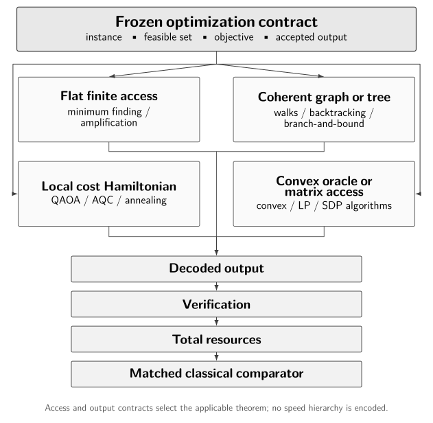
Frozen optimization contract branching through flat finite, coherent graph or tree, local cost Hamiltonian, and convex oracle or matrix access to a common verification and comparison path — Access and output contracts select which theorem is applicable; the diagram itself does not assert a speedup.

The branches are not a ranking. A problem may admit several interfaces, with different construction costs; price the reduction actually used.

A matched algorithm-selection table

Route	Required structure and access	Output	Guarantee regime	Hidden quantum cost	Matched classical comparator	Canonical owner
Unstructured minimum finding	Coherent values, comparisons, threshold updates, and verification over $N$ indices	Minimum index with bounded failure	$O(c\sqrt N)$ value queries for failure at most $2^{-c}$	Oracle construction, arithmetic, changing thresholds, memory, uncomputation	Explicit scan plus strongest applicable structured methods	Grover Search and Query Complexity
Amplitude-amplified feasible search	Coherent $A$ , inverse/reflection, good predicate, and marked weight $a$	Verified good candidate	Order $1/\sqrt a$ licensed attempts	Proposal preparation, reflections, rejection, unknown- $a$ schedule	Repeated proposal sampling with the same preparation information	Amplitude Amplification
Quantum walks or tree search	Reversible chain or coherent root, branch, predicate, and bound access	Detection, witness, or optimum after self-reduction	Spectral-walk or bounded-tree theorem under stated parameters	Setup/update, depth factors, reversible pruning, witness extraction	Same walk, backtracking, branch-and-bound, and preprocessing	Quantum Walk Algorithms
QAOA or variational optimization	Local cost, initial state, mixer, parameter and shot procedure	Samples and estimated objective statistics	Family- and depth-specific ideal or empirical result	Training, shots, restarts, compilation, selection bias, mitigation	Tuned local search, relaxations, heuristics, and exact methods on the same budget	QAOA and Variational Quantum Algorithms
Adiabatic quantum computation	Preparatory Hamiltonian, problem path, controls, relevant gap and schedule certificate	Final ground-subspace sample or decoded witness	Closed-system runtime/error theorem for the declared path	Path simulation/control, precision, coherence, preparation and readout	Classical exact/approximate solver and matched Hamiltonian simulation where relevant	Adiabatic Quantum Computation
Quantum annealing	Programmed driver/problem process, embedding, schedule, finite-time sampling	Decoded finite-time samples	Empirical time-to-target or scoped dynamical analysis	Programming, chains, gauges, reads, reset, decoding, rejected samples	Dated exact and heuristic portfolio including simulated annealing	Quantum Annealing
Convex, LP, or SDP oracle algorithms	Precise membership, separation, matrix, block, state, or sample access plus geometric bounds	Objective, decision, implicit state, or explicit vector as declared	Parameter-sensitive oracle or runtime theorem	Oracle construction, conditioning, precision, state preparation and output extraction	Same-oracle classical method or explicit-input solver with identical output	Quantum Linear Algebra and Block Encodings and QSVT

When a classical route remains the better claim

A classical route is better licensed when it matches the available input, output, or evidence more closely, even if a quantum theorem assumes a stronger oracle. Small or sparse structured instances may favor direct evaluation, dynamic programming, cuts, specialized branching, tensor networks, or approximation algorithms; explicit output can make readout decisive.

Classical algorithms also set the verification boundary. Exact solvers can provide bounds and proof artifacts; approximation algorithms can offer worst-case guarantees; heuristics can be tuned on the same distribution and budget. The correct comparator is not necessarily one method. It is a dated portfolio representing serious knowledge of the problem family, with preprocessing, warm starts, and selection effort counted symmetrically.

That conclusion concerns one frozen contract. Changes in access, accuracy, structure, hardware, or output can change the comparison, so version the record rather than generalizing it.

Quality Metrics, Repetitions, and Verification

Approximation metrics with valid denominators

Metric	Definition	Valid assumptions	Estimator or repetition rule	Common failure
Additive gap	$C_I(x)-C_I^*$ for feasible minimization	Same objective units and a known or bounded optimum	Candidate value minus certified reference; propagate reference uncertainty	Ignoring scale changes or constraint violation
Approximation ratio	$C_I(x)/C_I^*$ for nonnegative maximization	$C_I^*>0$ and a fixed zero of objective	Estimate candidate value and use a justified optimum or bound	Applying after arbitrary shifts or across sign changes
Target-hit probability	$\Pr[C_I(x)\le\tau,\ x\in\mathcal F(I)]$	Fixed target, decoder, and attempt distribution	Binomial or dependence-aware estimate; use the declared retry rule	Replacing hit rate with expected objective
Feasibility rate	$\Pr[x\in\mathcal F(I)]$ after decoding	Frozen constraints, tolerance, and decoder	Count accepted feasible outputs, including all rejections in cost	Reporting only postselected samples
Certified optimality gap	Feasible upper bound minus valid lower bound for minimization	Compatible primal/dual or search certificates	Recompute both bounds and their numerical residuals	Calling the gap to the best heuristic result certified
Time-to-solution	Total time to a verified target at stated confidence	Declared attempt dependence, success event, and full boundary	Combine setup and per-attempt terms with iid or conditional confidence	Using anneal or circuit time alone

Metrics answer different questions. Tie each reported metric to the accepted output; do not average unlike guarantees into one score.

Independent-run confidence and time-to-solution

If one independently verified run succeeds with probability $p_{\mathrm{tar}}$ and attempts are identically distributed and independent, the smallest number giving failure at most $\delta$ is

R = \left\lceil \frac{\ln\delta} {\ln(1-p_{\mathrm{tar}})} \right\rceil.

The edge cases are separate: if $p_{\mathrm{tar}}=0$ , no finite number of attempts reaches nonzero confidence; if $p_{\mathrm{tar}}=1$ , one attempt suffices. The formula assumes $0<p_{\mathrm{tar}}<1$ and $0<\delta<1$ . It also assumes that verification correctly identifies success.

If gauges, parameters, thresholds, incumbents, or device state adapt between attempts, use the declared conditional probabilities or a validated stopping process instead of the iid formula. Correlated hardware samples can make naive binomial confidence overoptimistic. A pilot estimate of $p_{\mathrm{tar}}$ carries uncertainty that should be propagated into a conservative repetition count.

Time-to-solution then includes fixed setup plus access construction, state preparation, coherent processing, measurement, decoding, verification, retry overhead, and parameter selection. Parallel execution changes wall time but not total work. Report both when the distinction affects the comparator.

Feasibility, certificates, and postselection

For an explicit bit string, verification may be cheap: inspect every local constraint and evaluate the objective. Optimality can be much harder, requiring a lower bound, exhaustive exclusion, or proof artifact. For LPs and SDPs, compatible primal and dual candidates can certify an objective interval, provided numerical residuals and sign conventions are checked. For an implicit quantum state, verification is usually statistical and observable-specific.

Postselection changes two things at once. It conditions the output distribution, and it reduces the probability that a preparation yields an accepted answer. Both the preselection and conditional statistics should be reported. Discarded infeasible samples still consume shots, anneals, readout, and decoder work. A repair heuristic creates a new decoded distribution and must be applied or priced comparably for classical methods.

Check decoded candidates against the original instance representation, not only the encoded coefficient table, and report tolerance and overflow rules.

Complete Resources, Comparators, and Evidence

One end-to-end cost boundary

A logical resource ledger includes input and oracle construction, logical data and work qubits, ancillas, controlled and inverse calls, objective and bound evaluations, non-Clifford gates, depth, coherent time, preparations, measurements, optimizer work, classical memory, repetitions, and output extraction. These are separate currencies until a cost model converts them. A query, shot, state preparation, and logical gate are not interchangeable units.

A fault-tolerant record adds code, logical-error target, physical errors, cycle time, routing, factories, parallelism, decoder latency, and uptime. An analog record adds control precision, embedding, calibration, programming, environment, timing, and rejections. Resource Estimation Tools owns physical lowering; this record states the boundary.

Costs can be amortized only under a declared workload. Building an oracle once for a million related instances differs from building it for one instance. Training reusable parameters, precomputing an embedding, or loading a database may likewise be amortized if the classical comparator receives the same repeated-use model.

A dated matched classical portfolio

A serious portfolio can contain exact enumeration, integer or mixed-integer programming, branch-and-bound and cutting planes, dynamic programming, local search, simulated annealing, semidefinite relaxations, approximation algorithms, tensor-network methods, and problem-specific heuristics. The set should reflect the instance family, not merely what is convenient to run. Software versions, hardware, parameter tuning, preprocessing, and stopping rules are dated evidence.

Matching requires the same instance distribution, warm starts, output type, tolerance, confidence, energy or hardware boundary, and selection budget. A quantum objective estimate should not be compared with a classical explicit optimizer. A quantum anneal interval should not be compared with classical end-to-end time. An assumed quantum oracle should be compared with the corresponding classical oracle model unless construction is charged to both.

Optimization Case Studies owns dated instances, executions, solver versions, scaling fits, and practical-advantage evidence. Algorithmic Benchmarking owns the general accepted-answer and cost-to-solution methodology. This page fixes the cross-route fields those studies must instantiate.

Evidence labels and licensed conclusions

Subject	Canonical owner	Retained here
Algorithmic primitives and query measures	Algorithmic Primitives and Query Complexity	Freeze the access and cost unit before choosing an optimization route
Unstructured search and amplification	Grover Search and Amplitude Amplification	Translate search guarantees to threshold and minimum-finding outputs
Quantum walks and tree search	Quantum Walk Algorithms	Compare coherent graph/tree access, decoded output, and pruning resources
Variational algorithms and QAOA	Variational Quantum Algorithms and QAOA	Separate expectation, sampled quality, training, and total selection cost
Adiabatic computation	Adiabatic Quantum Computation	Select the closed-system route under a licensed gap and schedule certificate
Quantum annealing	Quantum Annealing	Match finite-time samples, decoding, repetitions, and comparator boundary
Linear algebra and block-encoded primitives	Quantum Linear Algebra and Block Encodings and QSVT	Expose access, conditioning, output, and readout dependencies in optimization claims
Optimization case studies	Optimization Case Studies	Supply the timeless twelve-field schema used by dated studies
Benchmarking, resources, and evidence	Algorithmic Benchmarking, Resource Estimation Tools, and Claims, Hype, and Evidence Standards	Distinguish theorem, audit, demonstration, estimate, and end-to-end advantage

Use evidence labels literally. A theorem has formal assumptions; a finite audit checks specified arithmetic; a simulation covers a finite regime; a demonstration is hardware- and date-bound; a conditional estimate propagates a model; and an end-to-end benchmark compares complete procedures.

An oracle theorem does not establish implemented advantage, and a finite audit does not establish scaling. “No qualifying speedup is known” must name scope and review date; it is not a lower bound. Negative Results and Limitations retains the empirical ledger.

Three Reproducible Finite Audits

The three audits below are intentionally small enough to verify without a quantum software package. They test an encoding convention, an amplification probability and repetition ledger, and an optimization certificate plus output format. Every expected value is derived in prose before the script. Passing them establishes only these finite arithmetic contracts; it does not establish scaling, device performance, or quantum advantage.

Audit 1 — A penalty-QUBO and Ising map

Consider maximum-weight independent set on a triangle with weights $(3,2,2)$ . With $x_i=1$ meaning that vertex $i$ is selected, minimize

F_P(x) = -3x_0-2x_1-2x_2 + P(x_0x_1+x_1x_2+x_0x_2).

In lexicographic bit order, the first four strings are $000,001,010,011$ and the final four are $100,101,110,111$ ; direct evaluation at $P=4$ gives

(0,-2,-2,0,-3,-1,-1,5).

The unique minimum is $-3$ at $100$ . It is feasible because no edge has both endpoints selected. At $P=1$ , the corresponding values are

(0,-2,-2,-3,-3,-4,-4,-4).

The ground strings are $101$ , $110$ , and $111$ , all infeasible. Thus $P=4$ is strong enough and $P=1$ is too weak for this finite instance; enumeration proves no general penalty rule.

For $P=4$ , substitute $x_i=(1-z_i)/2$ . The three linear binary terms contribute the constant $-7/2$ and linear coefficients $(3/2,1,1)$ . Each of the three penalty terms contributes $1-z_i-z_j+z_iz_j$ , giving constant $3$ , linear contributions $(-2,-2,-2)$ , and unit pair couplings. Combining terms yields

F_4(z) = -\frac12 -\frac12z_0-z_1-z_2 +z_0z_1+z_1z_2+z_0z_2.

The constant, every linear coefficient, every pair coefficient, and all eight QUBO–Ising values are checked below.

Audit 2 — Threshold amplification and repetitions

Use the ordered table

(13,4,9,1,7,12,2,10,6,3,11,15,5,14,8,0)

and mark values strictly below $3$ . The marked entries are $1$ , $2$ , and $0$ , at zero-based indices $3$ , $6$ , and $15$ . Hence $N=16$ , $M=3$ , and $a=3/16$ . With $\theta=\arcsin\sqrt{3/16}$ , one Grover iterate has

\begin{aligned} p_1 &= \sin^2(3\theta)\\ &= \frac{243}{256}\\ &= 0.94921875. \end{aligned}

One attempt is below target confidence $0.99$ . Two independent attempts are minimal because

\begin{aligned} 1-\left(1-\frac{243}{256}\right)^2 &= \frac{65367}{65536}\\ &= 0.9974212646484375 > 0.99. \end{aligned}

Under the frozen primitive ledger, those two attempts use two independent uniform preparations, two threshold phase-oracle calls, two diffusion reflections, two measured candidates, and two classical verification evaluations. If access is instead a reversible value oracle, each threshold phase call requires a forward value computation and inverse uncomputation, for four value-oracle calls total. Comparison arithmetic and diffusion gates remain separate costs. This is one threshold subroutine, not a finite proof of the complete changing-threshold Dürr–Høyer schedule.

Audit 3 — A primal–dual certificate and output ledger

Take the primal linear program

\begin{aligned} \text{maximize}\quad & 3x+2y,\\ \text{subject to}\quad & x+y\le4,\\ & x\le2,\\ & y\le3,\\ & x,y\ge0. \end{aligned}

Under the convention established above, its dual is

\begin{aligned} \text{minimize}\quad & 4u+2v+3w,\\ \text{subject to}\quad & u+v\ge3,\\ & u+w\ge2,\\ & u,v,w\ge0. \end{aligned}

The primal vertices $(0,0)$ , $(2,0)$ , $(2,2)$ , $(1,3)$ , and $(0,3)$ have objective values $0$ , $6$ , $10$ , $9$ , and $6$ . Thus $(2,2)$ is the unique primal maximizer among the vertices. The dual point $(u,v,w)=(2,1,0)$ is feasible because $u+v=3$ and $u+w=2$ , and its objective is $4(2)+2(1)+3(0)=10$ . Weak duality gives every primal feasible value at most $10$ ; equality certifies both candidates as optimal.

Now freeze a classical output format. In two’s-complement $Q8.16$ , a $24$ -bit signed integer $k\in\{-2^{23},\ldots,2^{23}-1\}$ decodes as $k/2^{16}$ . The resolution is $2^{-16}$ and the representable interval is

[-128,\ 127.9999847412109375].

One scalar uses one sign bit, seven further integer bits, and sixteen fractional bits, totaling $24$ bits. An explicit ordered vector with $d_{\mathrm{out}}=4096$ coordinates uses

\begin{aligned} 4096(1+7+16) &= 98304\ \text{bits}\\ &= 12288\ \text{bytes}\\ &= 12\ \text{KiB}. \end{aligned}

Its payload is $4096$ times one scalar. A normalized amplitude state over $4096$ labels needs a $12$ -qubit address register, but it is not the same output as that ordered $98304$ -bit vector. This illustrative payload is not a query, tomography, or runtime lower bound.

"use strict";

const tolerance = 1e-12;
const assert = (condition, message) => {
  if (!condition) throw new Error(message);
};
const approx = (actual, expected, message) => {
  assert(Math.abs(actual - expected) <= tolerance, message);
};
const sameArray = (actual, expected, message) => {
  assert(
    actual.length === expected.length &&
      actual.every((value, index) => value === expected[index]),
    message,
  );
};

// Audit 1: enumerate the QUBO and verify the exact Ising substitution.
const strings = Array.from({ length: 8 }, (_, integer) => [
  (integer >> 2) & 1,
  (integer >> 1) & 1,
  integer & 1,
]);
const label = (x) => x.join("");
const feasibleIndependentSet = (x) =>
  x[0] * x[1] + x[1] * x[2] + x[0] * x[2] === 0;
const qubo = (x, penalty) =>
  -3 * x[0] -
  2 * x[1] -
  2 * x[2] +
  penalty * (x[0] * x[1] + x[1] * x[2] + x[0] * x[2]);
const groundLabels = (values) => {
  const minimum = Math.min(...values);
  return strings
    .filter((_, index) => values[index] === minimum)
    .map(label);
};

const valuesAtFour = strings.map((x) => qubo(x, 4));
const valuesAtOne = strings.map((x) => qubo(x, 1));
sameArray(valuesAtFour, [0, -2, -2, 0, -3, -1, -1, 5], "P=4 values");
sameArray(valuesAtOne, [0, -2, -2, -3, -3, -4, -4, -4], "P=1 values");
sameArray(groundLabels(valuesAtFour), ["100"], "P=4 ground set");
assert(Math.min(...valuesAtFour) === -3, "P=4 ground value");
assert(feasibleIndependentSet([1, 0, 0]), "P=4 feasibility");
sameArray(groundLabels(valuesAtOne), ["101", "110", "111"], "P=1 ground set");
assert(Math.min(...valuesAtOne) === -4, "P=1 ground value");
assert(
  groundLabels(valuesAtOne).every((bits) =>
    !feasibleIndependentSet(bits.split("").map(Number)),
  ),
  "all P=1 ground strings must be infeasible",
);

const isingCoefficients = {
  constant: -1 / 2,
  linear: [-1 / 2, -1, -1],
  pairs: { "01": 1, "12": 1, "02": 1 },
};
approx(isingCoefficients.constant, -0.5, "Ising constant");
sameArray(isingCoefficients.linear, [-0.5, -1, -1], "Ising linear terms");
sameArray(
  Object.values(isingCoefficients.pairs),
  [1, 1, 1],
  "Ising pair terms",
);
const isingAtFour = (x) => {
  const z = x.map((bit) => 1 - 2 * bit);
  return (
    isingCoefficients.constant +
    isingCoefficients.linear[0] * z[0] +
    isingCoefficients.linear[1] * z[1] +
    isingCoefficients.linear[2] * z[2] +
    isingCoefficients.pairs["01"] * z[0] * z[1] +
    isingCoefficients.pairs["12"] * z[1] * z[2] +
    isingCoefficients.pairs["02"] * z[0] * z[2]
  );
};
strings.forEach((x) => approx(isingAtFour(x), qubo(x, 4), "QUBO-Ising equality"));

// Audit 2: compute the marked fraction, rotation probability, and retry ledger.
const orderedValues = [13, 4, 9, 1, 7, 12, 2, 10, 6, 3, 11, 15, 5, 14, 8, 0];
const threshold = 3;
const markedIndices = orderedValues
  .map((value, index) => ({ value, index }))
  .filter(({ value }) => value < threshold)
  .map(({ index }) => index);
const population = orderedValues.length;
const markedCount = markedIndices.length;
const markedFraction = markedCount / population;
sameArray(markedIndices, [3, 6, 15], "marked indices");
assert(population === 16, "population");
assert(markedCount === 3, "marked count");
approx(markedFraction, 3 / 16, "marked fraction");
const theta = Math.asin(Math.sqrt(markedFraction));
approx(theta, Math.asin(Math.sqrt(3 / 16)), "theta");
const oneAttempt = Math.sin(3 * theta) ** 2;
approx(oneAttempt, 243 / 256, "one-iterate probability");
approx(oneAttempt, 0.94921875, "one-iterate decimal");
const confidenceAfter = (attempts) => 1 - (1 - oneAttempt) ** attempts;
let attempts = 1;
while (confidenceAfter(attempts) < 0.99) attempts += 1;
assert(confidenceAfter(1) < 0.99, "one attempt misses target");
assert(attempts === 2, "two attempts are minimal");
approx(confidenceAfter(2), 65367 / 65536, "two-attempt fraction");
approx(confidenceAfter(2), 0.9974212646484375, "two-attempt decimal");
const primitiveLedger = {
  uniformPreparations: attempts,
  thresholdPhaseCalls: attempts,
  diffusionReflections: attempts,
  measurements: attempts,
  classicalVerifications: attempts,
};
Object.values(primitiveLedger).forEach((count) =>
  assert(count === 2, "two-attempt primitive ledger"),
);
const reversibleValueOracleCalls = 2 * primitiveLedger.thresholdPhaseCalls;
assert(reversibleValueOracleCalls === 4, "value compute-uncompute ledger");

// Audit 3: verify primal-dual equality and the explicit-output payload.
const vertices = [
  [0, 0],
  [2, 0],
  [2, 2],
  [1, 3],
  [0, 3],
];
const primalFeasible = ([x, y]) =>
  x >= 0 && y >= 0 && x + y <= 4 && x <= 2 && y <= 3;
const primalObjective = ([x, y]) => 3 * x + 2 * y;
assert(vertices.every(primalFeasible), "primal vertices feasible");
const primalValues = vertices.map(primalObjective);
sameArray(primalValues, [0, 6, 10, 9, 6], "primal vertex values");
const primalOptimum = Math.max(...primalValues);
const primalMaximizers = vertices.filter(
  (vertex) => primalObjective(vertex) === primalOptimum,
);
assert(
  primalMaximizers.length === 1 &&
    primalMaximizers[0][0] === 2 &&
    primalMaximizers[0][1] === 2,
  "unique primal optimum",
);
assert(primalOptimum === 10, "primal optimum value");

const dual = { u: 2, v: 1, w: 0 };
assert(
  dual.u >= 0 &&
    dual.v >= 0 &&
    dual.w >= 0 &&
    dual.u + dual.v >= 3 &&
    dual.u + dual.w >= 2,
  "dual feasibility",
);
const dualValue = 4 * dual.u + 2 * dual.v + 3 * dual.w;
assert(dualValue === 10, "dual value");
assert(
  primalValues.every((value) => value <= dualValue),
  "finite weak-duality check",
);
assert(primalOptimum === dualValue, "primal-dual certificate");

const signBits = 1;
const furtherIntegerBits = 7;
const fractionalBits = 16;
const bitsPerCoordinate = signBits + furtherIntegerBits + fractionalBits;
const minimumInteger = -(2 ** 23);
const maximumInteger = 2 ** 23 - 1;
const resolution = 2 ** -fractionalBits;
const minimumValue = minimumInteger / 2 ** fractionalBits;
const maximumValue = maximumInteger / 2 ** fractionalBits;
assert(bitsPerCoordinate === 24, "Q8.16 word length");
approx(resolution, 2 ** -16, "Q8.16 resolution");
assert(minimumValue === -128, "Q8.16 minimum");
approx(maximumValue, 127.9999847412109375, "Q8.16 maximum");
const outputDimension = 4096;
const scalarBits = bitsPerCoordinate;
const vectorBits = outputDimension * bitsPerCoordinate;
const vectorBytes = vectorBits / 8;
const vectorKiB = vectorBytes / 1024;
const payloadRatio = vectorBits / scalarBits;
const addressQubits = Math.log2(outputDimension);
assert(scalarBits === 24, "scalar payload");
assert(vectorBits === 98304, "vector bit payload");
assert(vectorBytes === 12288, "vector byte payload");
assert(vectorKiB === 12, "vector KiB payload");
assert(payloadRatio === 4096, "vector-to-scalar payload ratio");
assert(addressQubits === 12, "address-register width");

console.log("Quantum-optimization finite audits: PASS");

Common Quantum-Optimization Claim Failures

Starting from NP-hardness. NP-hardness neither supplies an oracle nor implies a speedup. Begin with a represented family and accepted output, then name the theorem and comparator.

Calling a query count a runtime. Add value-circuit synthesis, loading, arithmetic, controls, inverse calls, verification, and readout before making a runtime claim.

Hiding an invalid ratio. Ratios need fixed signs and a nonzero denominator. If shifting the objective changes the headline, use a declared gap.

Treating mean energy as solution probability. Report target mass, feasibility, selected quality, and uncertainty separately from the mean.

Calling penalties and embeddings exact. Rounding, quadratization, embedding, chain decoding, and finite precision can alter results. Name each map and verify the executed objective.

Dropping the tree interface. Quote depth factors, logarithms, bound precision, witness recovery, and the classical tree definition alongside $\sqrt T$ .

Promoting scoped limitation results. A family-specific low-depth obstruction is not generic failure, and one favorable instance is not scalable advantage. Preserve both quantifiers.

Assuming an annealer samples Gibbs states. Record schedule, environment, gauges, embedding, decoding, and empirical distribution; finite-time dynamics need not be equilibrium.

Conflating implicit and explicit convex outputs. A state or objective estimate is not an explicit optimizer. Price coordinate extraction and certificate checks.

Comparing different cost boundaries. Match preprocessing, access, tuning, failures, confidence, output, verification, hardware, and amortization—not circuit time against classical wall time.

Exercises

1. Audit a QUBO–Ising map

For

F(x) = 2-5x_0+3x_1+6x_0x_1,

use $x_i=(1-z_i)/2$ to find the constant, both linear coefficients, and the pair coefficient in $F(z)$ . Verify the map on all four bit strings, including the constant term.

Solution

The substitutions are $-5x_0=-5/2+(5/2)z_0$ , $3x_1=3/2-(3/2)z_1$ , and

6x_0x_1 = \frac{6}{4}(1-z_0-z_1+z_0z_1).

The constants sum to $2-5/2+3/2+3/2=5/2$ . The $z_0$ coefficient is $5/2-3/2=1$ , the $z_1$ coefficient is $-3/2-3/2=-3$ , and the pair coefficient is $3/2$ . Therefore

F(z) = \frac52+z_0-3z_1+\frac32z_0z_1.

In bit order $00,01,10,11$ , the original values are $2,5,-3,6$ . Mapping bits to spins gives $(z_0,z_1)=(1,1),(1,-1),(-1,1),(-1,-1)$ , and the Ising expression yields the same four values. Omitting $5/2$ would preserve the ordering but fail the energy equality required by the contract.

2. Choose a safe penalty weight

Minimize $F_0(x)=-4x_0-3x_1$ subject to $x_0+x_1\le1$ . Encode the constraint with $G(x)=x_0x_1$ . Determine all $P$ for which $F_P=F_0+PG$ has only feasible ground strings. Test the borderline value explicitly.

Solution

The strings $00,01,10,11$ have unpenalized values $0,-3,-4,-7$ . The first three are feasible, and the best feasible value is $-4$ at $10$ . The infeasible string $11$ has penalized value $-7+P$ . To keep it strictly above the feasible optimum, require

-7+P>-4,

so $P>3$ . At $P=3$ , the infeasible string $11$ and feasible string $10$ both have value $-4$ ; therefore the ground space is not wholly feasible. Any $P>3$ makes $10$ the unique ground string. This exact answer uses the integer-valued violation $G\in\{0,1\}$ and does not transfer unchanged to another objective scale or encoding.

3. Separate expectation from target-hit probability

Let lower cost be better and let the target be $C\le1$ . Construct two distributions on costs $\{0,1,2,4\}$ with the same expected cost $2$ but different target-hit probabilities, one zero and one positive. Explain why an expectation-only optimization report cannot distinguish them.

Solution

Distribution $A$ puts probability one on cost $2$ . Its expectation is $2$ , and its target-hit probability is zero. Distribution $B$ puts probability $1/2$ on cost $0$ and probability $1/2$ on cost $4$ . Its expectation is also

\frac12(0)+\frac12(4)=2,

but its target-hit probability is $1/2$ because every cost- $0$ outcome is accepted. The distributions have identical means and sharply different best-of-budget behavior. With $R$ independent samples, $B$ hits the target with probability $1-2^{-R}$ , whereas $A$ never does. An expectation report must therefore be supplemented by the acceptance event, its estimated probability, and the sampling budget whenever the application wants a candidate rather than a mean.

4. Count threshold-amplification repetitions

For the finite threshold audit above, derive $p_1=243/256$ from $a=3/16$ without decimal rounding. Then find the smallest number of independent attempts needed for confidence at least $0.99$ , and give the exact confidence.

Solution

Let $\sin\theta=\sqrt3/4$ and $\cos\theta=\sqrt{13}/4$ . The triple-angle identity gives

\sin(3\theta) = 3\sin\theta-4\sin^3\theta = \frac{3\sqrt3}{4}-\frac{3\sqrt3}{16} = \frac{9\sqrt3}{16}.

Squaring yields $p_1=243/256$ . One attempt has confidence $0.94921875<0.99$ . Two attempts have

1-\left(\frac{13}{256}\right)^2 = 1-\frac{169}{65536} = \frac{65367}{65536} = 0.9974212646484375.

Thus two are minimal. Under the stated ledger they cost two phase-oracle calls, or four value-oracle calls when each phase oracle is built by compute–phase–uncompute.

5. Compare flat search with a pruned tree

A problem has $N=2^{40}$ candidate strings. A declared classical branch-and-bound procedure explores $T=2^{18}$ vertices to depth $d=40$ . Compare the leading flat minimum-finding count $\sqrt N$ with the leading backtracking expression $\sqrt T\,d^{3/2}\log_2d$ . Assume one flat value query costs $q_v$ logical gates and one coherent tree test costs $q_t$ . State the inequality under which the tree route has the smaller displayed logical-gate ledger, and explain what this comparison cannot prove.

Solution

The flat leading count is $\sqrt N=2^{20}=1{,}048{,}576$ value queries. The tree expression is

\sqrt T\,d^{3/2}\log_2d = 2^9(40)^{3/2}\log_2 40 \approx 6.89\times10^5

coherent tests, before hidden constants and additional logarithms. Under only these displayed terms, the tree route has the smaller logical-gate ledger when

(6.89\times10^5)q_t < (1.048576\times10^6)q_v,

or approximately $q_t<1.52q_v$ . The numerical comparison does not prove an end-to-end speedup: it omits exact theorem constants, reversible branching and witness recovery, memory, error correction, output verification, and alternative classical solvers. It also treats the declared classical tree size as fixed; better pruning or variable ordering could change $T$ .

6. Verify a primal–dual certificate

For the LP in Audit 3, verify primal feasibility of $(2,2)$ and dual feasibility of $(2,1,0)$ . Derive the weak-duality inequality directly and conclude optimality without enumerating vertices.

Solution

The primal point obeys $2+2=4$ , $2\le2$ , $2\le3$ , and nonnegativity. Its objective is $3(2)+2(2)=10$ . The dual point is nonnegative and obeys $u+v=3$ and $u+w=2$ , so its objective is $4(2)+2(1)+3(0)=10$ .

For any primal-feasible $(x,y)$ and dual-feasible $(u,v,w)$ ,

\begin{aligned} 3x+2y &\le (u+v)x+(u+w)y\\ &=u(x+y)+vx+wy\\ &\le4u+2v+3w. \end{aligned}

The first inequality uses the dual constraints and $x,y\ge0$ ; the last uses the primal constraints and $u,v,w\ge0$ . Thus every primal objective is at most every dual objective. Equality at the two candidates proves both optimal, with zero primal–dual gap.

7. Repair a quantum-SDP speedup claim

Repair the statement “The quantum SDP solver is exponentially faster because it depends logarithmically on matrix dimension.” Write a claim that is testable and does not exceed the cited oracle theorems or lower bounds.

Solution

A repaired claim might read: “For the specified family of $m$ -constraint, $n$ -dimensional SDPs, assuming the paper’s sparse or quantum input oracle at precision $\eta$ , bounded operator norms and width $W$ , feasibility promise, and failure probability $\delta$ , the named algorithm returns an $\epsilon$ -additive objective estimate (not an explicit primal matrix) with the theorem’s full dependence on $m,n,\epsilon,\eta,W$ , sparsity, and solution bounds. We will implement or separately price oracle construction, state preparation, and verification, and compare against a dated classical solver using the same represented input and scalar output.”

One should then instantiate the actual bound rather than retaining the phrase “depends logarithmically.” The worst-case lower-bound regimes with $\Omega(mn)$ complexity when $m$ is comparable to $n$ rule out a universal dimension-only exponential claim in the cited model. A favorable structured regime may remain possible, but it needs a complete parameter and output record.

8. Build a matched optimization claim record

A study reports: “A depth- $3$ QAOA circuit found a good portfolio on 20 assets using 20 qubits and 10,000 shots, beating simulated annealing.” Identify the missing information in all twelve fields and give a minimally complete replacement claim.

Solution

The statement omits the family and effective size after encoding; asset data, distribution, and promises; variables, budget and risk constraints; objective units and coefficient precision; data-to-Hamiltonian construction; output decoder; the definition of “good,” tolerance, and confidence; mixer, initial state, angle domain, optimizer, seeds, and compilation; per-run success, independent evaluation, retries, and stopping; training, rejected shots, classical work, and physical time; simulated-annealing implementation, tuning, hardware, and full boundary; and the evidence label.

A minimally complete replacement is: “On the frozen set of named 20-asset instances dated YYYY-MM-DD, encoded as $n$ binary allocation variables with the listed budget and risk constraints and fixed-point coefficients, depth- $3$ QAOA used the stated feasible initial state, mixer, angle ranges, optimizer, five seeds, and shot allocation. It returned decoded feasible bit strings; success meant objective at most the preregistered threshold $\tau$ . Independent evaluation shots estimated target probability with the stated confidence interval. The ledger includes Hamiltonian construction, compilation, every training and evaluation circuit, rejected samples, decoding, verification, and wall time. A versioned simulated-annealing portfolio received the same encoded instances, tuning budget, output threshold, confidence target, hardware boundary, and preprocessing. The evidence is a finite benchmark on these instances; it establishes neither asymptotic nor practical advantage beyond this scope.”

References

Dorit Aharonov, Wim van Dam, Julia Kempe, Zeph Landau, Seth Lloyd, and Oded Regev, “Adiabatic Quantum Computation Is Equivalent to Standard Quantum Computation,” SIAM Journal on Computing 37(1), 166–194 (2007), doi:10.1137/S0097539705447323.
Charles H. Bennett, Ethan Bernstein, Gilles Brassard, and Umesh Vazirani, “Strengths and Weaknesses of Quantum Computing,” SIAM Journal on Computing 26(5), 1510–1523 (1997), doi:10.1137/S0097539796300933.
Gilles Brassard, Peter Høyer, Michele Mosca, and Alain Tapp, “Quantum Amplitude Amplification and Estimation,” Contemporary Mathematics 305, 53–74 (2002), doi:10.1090/conm/305/05215.
Sergey Bravyi, Alexander Kliesch, Robert Koenig, and Eugene Tang, “Obstacles to Variational Quantum Optimization from Symmetry Protection,” Physical Review Letters 125, 260505 (2020), doi:10.1103/PhysRevLett.125.260505.
Christoph Dürr and Peter Høyer, “A Quantum Algorithm for Finding the Minimum,” arXiv:quant-ph/9607014 (1996), arXiv:quant-ph/9607014.
Edward Farhi, David Gamarnik, and Sam Gutmann, “The Quantum Approximate Optimization Algorithm Needs to See the Whole Graph: Worst Case Examples,” arXiv:2005.08747 (2020), arXiv:2005.08747.
Edward Farhi, Jeffrey Goldstone, and Sam Gutmann, “A Quantum Approximate Optimization Algorithm,” arXiv:1411.4028 (2014), arXiv:1411.4028.
Edward Farhi, Jeffrey Goldstone, Sam Gutmann, Joshua Lapan, Andrew Lundgren, and Daniel Preda, “A Quantum Adiabatic Evolution Algorithm Applied to Random Instances of an NP-Complete Problem,” Science 292(5516), 472–475 (2001), doi:10.1126/science.1057726.
Michel X. Goemans and David P. Williamson, “Improved Approximation Algorithms for Maximum Cut and Satisfiability Problems Using Semidefinite Programming,” Journal of the ACM 42(6), 1115–1145 (1995), doi:10.1145/227683.227684.
Lov K. Grover, “A Fast Quantum Mechanical Algorithm for Database Search,” Proceedings of the Twenty-Eighth Annual ACM Symposium on Theory of Computing, 212–219 (1996), doi:10.1145/237814.237866.
Stuart Hadfield, Zhihui Wang, Bryan O’Gorman, Eleanor G. Rieffel, Davide Venturelli, and Rupak Biswas, “From the Quantum Approximate Optimization Algorithm to a Quantum Alternating Operator Ansatz,” Algorithms 12(2), 34 (2019), doi:10.3390/a12020034.
M. B. Hastings, “Classical and Quantum Bounded Depth Approximation Algorithms,” Quantum Information and Computation 19(13–14), 1116–1140 (2019), doi:10.26421/QIC19.13-14-3.
Tadashi Kadowaki and Hidetoshi Nishimori, “Quantum Annealing in the Transverse Ising Model,” Physical Review E 58, 5355–5363 (1998), doi:10.1103/PhysRevE.58.5355.
Frédéric Magniez, Ashwin Nayak, Jérémie Roland, and Miklos Santha, “Search via Quantum Walk,” SIAM Journal on Computing 40(1), 142–164 (2011), doi:10.1137/090745854.
Ashley Montanaro, “Quantum-Walk Speedup of Backtracking Algorithms,” Theory of Computing 14(15), 1–24 (2018), doi:10.4086/toc.2018.v014a015.
Ashley Montanaro, “Quantum Speedup of Branch-and-Bound Algorithms,” Physical Review Research 2, 013056 (2020), doi:10.1103/PhysRevResearch.2.013056.
Troels F. Rønnow, Zhihui Wang, Joshua Job, Sergio Boixo, Sergei V. Isakov, David Wecker, John M. Martinis, Daniel A. Lidar, and Matthias Troyer, “Defining and Detecting Quantum Speedup,” Science 345(6195), 420–424 (2014), doi:10.1126/science.1252319.
Joran van Apeldoorn, András Gilyén, Sander Gribling, and Ronald de Wolf, “Convex Optimization Using Quantum Oracles,” Quantum 4, 220 (2020), doi:10.22331/q-2020-01-13-220.
Joran van Apeldoorn, András Gilyén, Sander Gribling, and Ronald de Wolf, “Quantum SDP-Solvers: Better Upper and Lower Bounds,” Quantum 4, 230 (2020), doi:10.22331/q-2020-02-14-230.
Christof Zalka, “Grover’s Quantum Searching Algorithm Is Optimal,” Physical Review A 60, 2746–2751 (1999), doi:10.1103/PhysRevA.60.2746.