Quantum Phase Estimation

Short Definition

Quantum phase estimation (QPE) estimates an eigenphase of a unitary operator. Given

$$U\lvert u\rangle = e^{2\pi i\phi}\lvert u\rangle, \qquad 0\leq\phi<1,$$

standard QPE uses controlled powers of $U$, phase kickback, and an inverse quantum Fourier transform to return an $m$-bit estimate of $\phi$.

QPE is not merely a way to read a phase already attached to an isolated state. An overall phase is unobservable. Controlled evolution converts the eigenphase into relative phases on a control register, where interference can reveal it. The algorithm is central to order finding, energy estimation, quantum counting, amplitude estimation, and many spectral algorithms.

This page is the canonical home for the eigenphase problem, the standard circuit, its exact probability law, precision guarantees, iterative variants, and resource accounting. The dedicated Phase Kickback page owns the general phase-transduction contract, while Algorithmic Primitives owns the broader algorithm-composition language.

The Eigenphase Contract

The ideal input contract contains more than the equation $U\lvert u\rangle=e^{2\pi i\phi}\lvert u\rangle$:

1. a procedure prepares the eigenstate $\lvert u\rangle$, or a state with stated overlap on relevant eigenspaces;
2. controlled implementations of $U^{2^j}$ are available for the required integers $j$;
3. the phase convention and interval are fixed;
4. a target accuracy and failure probability are specified;
5. the cost model says whether powers are primitive calls, repeated base operations, or simulated evolution for longer times.

These assumptions determine whether QPE is useful. The inverse Fourier transform can be modest compared with preparing a good eigenstate or implementing the largest controlled power.

Phase is defined modulo one

The eigenvalue determines

$$\phi\pmod 1.$$

QPE cannot distinguish $\phi$ from $\phi+\ell$ for integer $\ell$. For Hamiltonian energies, this becomes an aliasing interval that must be resolved using an energy promise, an offset, or several evolution times.

Controlled access is a separate capability

An uncontrolled implementation of $U$ does not automatically supply a cheap controlled-$U$. The controlled operation must preserve a coherent distinction between “apply $U$” and “do nothing.” If $U$ is given as a known gate sequence, its gates can often be controlled with additional synthesis cost. If $U$ is generated by a Hamiltonian, a controlled simulation protocol must be designed.

This distinction also fixes the phase origin. Replacing $U$ by $e^{i\alpha}U$ changes no unconditional experiment, but controlled-$U$ makes $e^{i\alpha}$ a relative phase on the control. The physical implementation, not only the abstract channel induced by $U$, therefore matters.

Controlled Operations owns the generic semantic and evidence audit for that access assumption; this page retains the powered-access contract, phase-estimation algorithm, precision guarantees, and resource costs.

Phase Kickback from Powered Unitaries

Phase Kickback owns the base common-eigenstate identity, target-return test, relative-phase convention, and phase-sensitive readout. This section specializes that licensed mechanism to powered unitaries, a multi-qubit phase-gradient register, and the precision and resource obligations of QPE.

Begin with one control qubit in $\lvert+\rangle$ and the target eigenstate:

$$\frac{\lvert0\rangle+\lvert1\rangle}{\sqrt2} \otimes \lvert u\rangle.$$

A controlled-$U^k$ produces

$$\frac{ \lvert0\rangle + e^{2\pi i k\phi}\lvert1\rangle }{\sqrt2} \otimes \lvert u\rangle.$$

The target returns to the same eigenstate. Its eigenphase has become a measurable relative phase on the control. Using powers $k=1,2,4,\ldots$ interrogates successively finer binary scales of $\phi$.

For $m$ control qubits, let the computational-basis integer be

$$k = \sum_{j=0}^{m-1}k_j2^j.$$

Prepare every control in $\lvert+\rangle$ and apply controlled-$U^{2^j}$ from control $j$. The joint state becomes

$$\begin{aligned} \lvert\Psi_\phi\rangle &= \frac1{\sqrt{2^m}} \sum_{k=0}^{2^m-1} \lvert k\rangle U^k\lvert u\rangle \\ &= \frac1{\sqrt{2^m}} \sum_{k=0}^{2^m-1} e^{2\pi i k\phi} \lvert k\rangle\lvert u\rangle. \end{aligned}$$

The control register is a discrete phase-gradient state. The target factors out because it is an eigenstate.

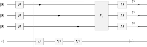
For three control qubits, controlled $U$, $U^2$, and $U^4$ encode the eigenphase at binary scales. The inverse QFT concentrates the phase gradient into an estimate $y/8$; the target eigenstate is preserved ideally.

The Inverse Quantum Fourier Transform

Let $L=2^m$. The Quantum Fourier Transform page owns the circuit construction, swaps, abstract resource count, and approximation cutoff. This page fixes the convention used by the phase decoder:

$$F_L\lvert y\rangle = \frac1{\sqrt L} \sum_{k=0}^{L-1} e^{2\pi i ky/L} \lvert k\rangle.$$

If the phase has an exact $m$-bit representation,

$$\phi=\frac aL, \qquad a\in\{0,1,\ldots,L-1\},$$

then the control state is exactly $F_L\lvert a\rangle$. Applying $F_L^\dagger$ gives

$$F_L^\dagger \left( \frac1{\sqrt L} \sum_{k=0}^{L-1} e^{2\pi i k\phi}\lvert k\rangle \right) = \lvert a\rangle.$$

Measurement returns the binary digits of $a$ with certainty in the ideal circuit.

Different circuit diagrams reverse qubit order or attach $U^{2^j}$ to wires in the opposite vertical order. Some QFT circuits include explicit final swaps; others absorb bit reversal into classical interpretation. The safe convention is to define the integer $k$, the Fourier sign, and the output bit order algebraically.

The QFT is a decoder, not a spectrum dump

The inverse QFT converts one coherently encoded phase into a concentrated measurement distribution. It does not print a classical list of all eigenphases or Fourier coefficients. One run returns one $m$-bit string.

An exact inverse QFT on $m$ qubits uses order $m^2$ one- and two-qubit gates in the standard decomposition. Small controlled rotations can be omitted in an approximate QFT, reducing gate count while adding a controlled approximation error. The classical fast Fourier transform is related mathematically but acts on an explicitly stored classical vector and has a different input-output contract.

The Probability Distribution for an Inexact Phase

Most phases are not exactly representable with $m$ bits. After the inverse QFT, the amplitude of outcome $y$ is

$$\begin{aligned} a_y &= \frac1L \sum_{k=0}^{L-1} e^{2\pi i k\delta_y}, \\ \delta_y &= \phi-\frac yL. \end{aligned}$$

Summing the geometric series gives

$$a_y = e^{\pi i(L-1)\delta_y} \frac{ \sin(\pi L\delta_y) }{ L\sin(\pi\delta_y) },$$

with the continuous limit $a_y=1$ when $\delta_y=0$. Therefore

$$\Pr(Y=y) = \frac{ \sin^2(\pi L\delta_y) }{ L^2\sin^2(\pi\delta_y) }.$$

This is a periodic finite-resolution kernel sharply peaked near $y\approx L\phi$. Its side lobes are real algorithmic probability, not numerical noise.

Nearest-bin guarantee

Let $y_\star$ be the integer nearest to $L\phi$, interpreted around the phase circle. Then

$$\lvert\delta_{y_\star}\rvert \leq \frac1{2L}.$$

Using elementary sine bounds in the probability formula gives

$$\Pr(Y=y_\star) \geq \frac4{\pi^2} \approx0.405.$$

This lower bound is conservative. Repetition raises confidence, and retaining nearby outcomes can give a larger useful success probability.

Guard bits

Suppose the goal is $n$ bits of phase accuracy with failure probability at most $\epsilon$. A standard sufficient choice is to run QPE with

$$m = n+ \left\lceil \log_2\!\left( 2+\frac1{2\epsilon} \right) \right\rceil$$

control qubits, then round or discard the extra low-significance bits. The added bits narrow the Fourier kernel relative to the requested $n$-bit bin. The bound is sufficient rather than always tight; an application should state its exact acceptance interval and postprocessing.

Worked Examples

An exactly representable phase

Take

$$\phi=\frac58=0.101_2$$

and $m=3$. After controlled powers, the control state is

$$\frac1{\sqrt8} \sum_{k=0}^{7} e^{2\pi i5k/8}\lvert k\rangle = F_8\lvert5\rangle.$$

The inverse QFT produces

$$\lvert5\rangle=\lvert101\rangle$$

with probability one, subject to the chosen output-bit convention.

A phase between binary grid points

Let $\phi=0.3$ and $m=3$, so $L=8$. The nearest grid points are $2/8=0.25$ and $3/8=0.375$. The probability formula gives approximately

$$\begin{aligned} \Pr(Y=2) &\approx0.578, \\ \Pr(Y=3) &\approx0.259. \end{aligned}$$

The two nearest outcomes together carry about $0.837$ probability. Reporting only the mode $2/8$ gives an error of $0.05$; retaining the full likelihood conveys the finite-resolution uncertainty more honestly.

Input States That Are Not Eigenstates

Suppose the target is

$$\lvert\psi\rangle = \sum_j c_j\lvert u_j\rangle, \qquad U\lvert u_j\rangle = e^{2\pi i\phi_j}\lvert u_j\rangle.$$

Linearity gives, schematically,

$$\lvert0^m\rangle\lvert\psi\rangle \longmapsto \sum_j c_j \lvert\widetilde{\phi_j}\rangle \lvert u_j\rangle,$$

where $\lvert\widetilde{\phi_j}\rangle$ denotes the finite-resolution estimate distribution centered on $\phi_j$. Measuring the control samples eigenphase $j$ with probability approaching $\lvert c_j\rvert^2$ when the peaks are well resolved. The target is correspondingly projected toward the associated eigenspace.

Consequences:

• QPE does not preferentially find the ground state unless the input has substantial ground-state overlap.
• An eigenvalue absent from the input state cannot appear.
• Degenerate eigenvectors sharing one phase are not distinguished; the measurement projects onto their common eigenspace.
• Eigenphases separated by less than the achieved resolution produce overlapping distributions.
• Repeating until a rare eigenvalue appears costs order $1/\lvert c_j\rvert^2$ state preparations unless another coherent amplification mechanism is available.

This is an approximate implementation of the spectral-measurement logic developed in Spectral Decomposition and Projective Measurement.

Precision Costs Time

An $m$-qubit control register requires powers through

$$U^{2^{m-1}}.$$

There are only $m$ distinct controlled-power blocks, but that statement can hide their cost.

Three access models

Access model	Cost assigned to $U^{2^j}$	Consequence
powered-unitary oracle	one primitive call	strong model; the power oracle itself needs justification
repeated base unitary	$2^j$ calls to $U$	total base calls are $2^m-1$
Hamiltonian evolution	simulate time $2^j\tau$	cost normally grows with evolution time, norm, and target error

Quantum Oracles owns the declaration of whether base, inverse, controlled, or powered unitary access is supplied and which conversions are licensed. QPE owns the phase gradient, precision and success guarantees, decoder, and coherent-time costs once that access record is fixed.

The Quantum Algorithms and Complexity chapter guide records three powered calls, seven repetition-equivalent base-$U$ interrogation units, maximum individual block duration four, and a standard-circuit coherent horizon of at least seven interrogation units plus decoding and other gates; these are not interchangeable resource statements.

Treating every $U^{2^j}$ as one elementary gate can create a fictitious exponential speedup. In order finding, modular arithmetic supplies efficient structured implementations of the powers. In energy estimation, long-time dynamics generally carry a correspondingly long physical or logical cost.

Total interrogation time

If

$$U=e^{-iH\tau},$$

then $U^{2^j}$ is evolution for time $2^j\tau$. The sum of controlled evolution times is

$$T_{\mathrm{tot}} = \tau\sum_{j=0}^{m-1}2^j = (2^m-1)\tau.$$

The phase resolution is order $2^{-m}$, so the energy resolution scales as order $1/T_{\mathrm{tot}}$, up to constants and algorithmic errors. QPE trades coherent evolution time for spectral resolution; the $m$-bit output does not arise from only polynomial interrogation time in $m$.

Gate and error budget

A complete error budget separates:

• target-state preparation error and eigenstate overlap;
• controlled-simulation error for each power;
• coherent over-rotations and phase bias;
• inverse-QFT approximation error;
• decoherence during the longest controlled evolution;
• measurement and feedforward errors;
• statistical failure from the finite-resolution distribution.

Errors in the largest powers are especially consequential because they encode the finest phase information. Synthesis cost for small inverse-QFT rotations may also be significant in a fault-tolerant gate set. Universal Gate Sets supplies that logical-to-native distinction.

Energy Estimation and Aliasing

For a Hamiltonian eigenstate,

$$H\lvert E\rangle = E\lvert E\rangle,$$

time evolution gives

$$e^{-iH\tau}\lvert E\rangle = e^{-iE\tau}\lvert E\rangle.$$

Thus QPE can estimate $E\tau$ only modulo $2\pi$. If a promised spectral interval is $E_{\min}\leq E\leq E_{\max}$, a convenient shifted unitary is

$$U = e^{-i(H-E_{\max}I)\tau}.$$

Its phase is

$$\phi_E = \frac{(E_{\max}-E)\tau}{2\pi}$$

without wrapping provided

$$(E_{\max}-E_{\min})\tau<2\pi.$$

The energy can then be reconstructed as

$$E = E_{\max} - \frac{2\pi\phi_E}{\tau}.$$

A smaller $\tau$ increases the unambiguous energy range but worsens the energy represented by one phase bin. A larger maximum evolution time improves resolution. Selecting $\tau$, the offset, and $m$ is therefore one coupled design problem.

The Time-Evolution Operator fixes the physical sign convention. Product formulas are one possible implementation route: Trotter Product Formula derives the operator splitting, while Trotter–Suzuki Methods treats controlled-circuit cost and the resulting eigenphase or energy bias.

Iterative and Semiclassical Variants

The standard circuit stores all phase bits coherently and then applies an inverse QFT. Several variants trade qubit count against repetitions, feedback, and coherent duration.

Semiclassical inverse QFT

When the QFT is immediately followed by computational-basis measurement, controlled rotations within the inverse QFT can be replaced by sequential single-qubit measurements and classically controlled phase corrections. This is the Griffiths–Niu semiclassical Fourier transform.

It removes entangling gates from the final Fourier decoder and can permit control-qubit reuse. It does not remove the need for powered controlled-$U$ operations, a coherent target, or accurate feedforward.

Single-ancilla iterative phase estimation

Iterative QPE reuses one control qubit. Each round applies a selected controlled power, adds a phase correction determined by previously inferred bits, and measures the control. The target eigenstate is retained for the next round or prepared again.

The width falls from $m$ control qubits to one, but:

• rounds are sequential;
• mid-circuit measurement and low-latency feedforward are required;
• an early bit error can corrupt later corrections;
• the largest controlled power and total interrogation time remain;
• repeated shots may be needed to make each bit reliable.

The two-qubit implementation studied by Dobšíček and collaborators is a standard concrete form of this idea.

Kitaev-style statistical estimation

One-control experiments can estimate the quadratures of

$$e^{2\pi i k\phi}$$

for selected integers $k$. A Hadamard test measures cosine; adding a quarter-cycle phase shift measures sine. Classical reconstruction combines these noisy modular-angle estimates.

This approach avoids a coherent multi-qubit inverse QFT and supports flexible statistical inference. It replaces coherent width with repeated experiments and a nontrivial phase-unwrapping problem. Bayesian, maximum-likelihood, and robust phase-estimation protocols refine this tradeoff for particular noise and prior-information models.

No variant makes precision free. They redistribute control qubits, circuit depth, shots, classical processing, and tolerance to noise.

Roles in Larger Algorithms

Order finding and Shor’s algorithm

For modular multiplication, relevant unitary eigenphases are rational numbers of the form

$$\phi=\frac sr.$$

QPE samples an approximation to $s/r$, and continued fractions can recover the order $r$ when the precision and number-theoretic conditions are sufficient. The input need not be one known eigenstate; it decomposes into eigenstates whose phases are sampled.

The crucial implementation fact is that controlled powers of modular multiplication can be built by repeated squaring and reversible arithmetic. They are not realized by naively repeating one enormous circuit $2^j$ times. QPE supplies period information, while the reduction from factoring to order finding, arithmetic, success analysis, and classical postprocessing belong to the full Shor Algorithm.

Quantum chemistry and many-body spectra

Set $U$ to a simulated time-evolution operator and prepare a trial state with overlap on a molecular or many-body eigenstate. QPE can estimate the corresponding energy and project the target toward that eigenspace.

The difficult resources are often:

• preparing a sufficiently accurate trial state;
• simulating controlled dynamics for long times;
• resolving nearby levels;
• repeating when the desired overlap is small;
• implementing the algorithm fault tolerantly.

The phase-estimation subroutine alone does not establish an end-to-end speedup over the best classical method. Simulation of Quantum Chemistry and Simulation of Quantum Materials place these dependencies inside molecular and periodic or effective-model workflows, respectively. Quantum Algorithms for Chemistry and Materials compares this overlap- and precision-sensitive spectral route with variational and direct-dynamics alternatives; this page retains the generic phase-estimation kernel and coherent-time requirements.

Simulation, counting, and spectral transforms

QPE appears whenever useful information is encoded in a unitary eigenphase:

• Hamiltonian simulation supplies $e^{-iHt}$ so energies become phases.
• Quantum counting applies QPE to the Grover iterate, whose rotation angle encodes the number of marked items.
• Amplitude Estimation reuses this page’s generic single-phase kernel and powered circuit, then owns the conjugate Grover eigenphase mixture, the $\sin^2$ decoder, probability-error bound, and complete component ledger.
• Linear-system and spectral algorithms condition rotations or filters on estimated eigenvalues.
• Eigenstate filtering and projection use the phase register as a spectral label.

Hamiltonian Simulation specifies the access, normalization, controlled-query, energy-offset, and simulation-error contracts behind that first bullet. Those costs must be combined with the overlap, resolution, and decoding costs developed here. Qubitization and Quantum Signal Processing explains the alternative of phase-estimating a qubitized walk directly, including the two eigenphase branches and the conversion $E=\alpha\cos\theta_E$. Simulation of Quantum Chemistry connects those phase and simulation contracts to molecular integral conventions, active spaces, fermion encodings, state overlap, and chemical error budgets.

These compositions require more than citing QPE by name. Each must state how the eigenstate overlap, controlled powers, phase precision, and readout error enter the final task.

Common Mistakes

• Saying QPE measures an unobservable global phase. Controlled evolution makes an eigenphase relative to a reference branch.
• Assuming any unknown black-box unitary can be controlled at no cost.
• Counting $m$ powered-unitary blocks while ignoring their exponents or evolution times.
• Claiming $m$ output bits imply only polynomial cost in $m$.
• Expecting a deterministic bit string when $\phi$ is not on the $m$-bit grid.
• Feeding an arbitrary state into QPE and calling the result its expectation value. QPE samples spectral components instead.
• Assuming QPE prepares the ground state even when the trial overlap is tiny.
• Ignoring phase wraparound when converting a phase to energy.
• Mixing Fourier-sign, wire-order, and binary-endianness conventions.
• Treating the inverse QFT as a classical readout of an entire spectrum.
• Reporting algorithmic precision without simulation, synthesis, decoherence, and failure-probability errors.

Resource Checklist

Before using QPE, record:

1. the unitary and eigenphase convention;
2. the state-preparation method and relevant eigenstate overlaps;
3. how controlled-$U^{2^j}$ is implemented;
4. the largest power, total evolution time, and gate count;
5. the phase interval, aliasing promise, and output-bit order;
6. target accuracy and total failure probability;
7. inverse-QFT or iterative-decoder approximation;
8. simulation, synthesis, noise, and measurement errors;
9. the classical postprocessing and final application output.

This is the phase-estimation specialization of the resource ledger in Claims, Hype, and Evidence Standards.

Exercises

1. Exact three-bit phase

Let $\phi=5/8$ and use three control qubits. Show directly that the phase-gradient state equals $F_8\lvert5\rangle$ and give the measured bit string after the inverse QFT.

Solution

The control state before the inverse QFT is

$$\frac1{\sqrt8} \sum_{k=0}^{7} e^{2\pi i k(5/8)} \lvert k\rangle.$$

By the stated Fourier convention, this is exactly $F_8\lvert5\rangle$. Therefore

$$F_8^\dagger F_8\lvert5\rangle = \lvert5\rangle = \lvert101\rangle.$$

If a circuit omits final swaps, its physical wire order may display the reversed string; the decoded integer remains $5$ after applying the declared convention.

2. Derive the phase-gradient state

Starting from $\lvert+\rangle^{\otimes m}\lvert u\rangle$, prove that controlled powers $U^{2^j}$ produce

$$\frac1{\sqrt{2^m}} \sum_{k=0}^{2^m-1} e^{2\pi i k\phi} \lvert k\rangle\lvert u\rangle.$$

Solution

Write a control string as $k_0k_1\ldots k_{m-1}$ with integer

$$k=\sum_{j=0}^{m-1}k_j2^j.$$

On that branch, control $j$ applies $U^{2^j}$ only when $k_j=1$. The total target operation is

$$\prod_{j=0}^{m-1} U^{k_j2^j} = U^k.$$

Because $\lvert u\rangle$ is an eigenstate,

$$U^k\lvert u\rangle = e^{2\pi i k\phi}\lvert u\rangle.$$

Summing over the $2^m$ equally weighted control strings gives the stated result.

3. Nearest-bin lower bound

Let $y_\star$ be nearest to $L\phi$, so $\lvert\delta\rvert\leq1/(2L)$. Use

$$\sin x\geq\frac{2x}{\pi}$$

for $0\leq x\leq\pi/2$ and $\sin x\leq x$ for $x\geq0$ to prove $\Pr(Y=y_\star)\geq4/\pi^2$.

Solution

By symmetry take $\delta\geq0$. Since $\pi L\delta\leq\pi/2$,

$$\sin(\pi L\delta) \geq 2L\delta.$$

Also,

$$L\sin(\pi\delta) \leq \pi L\delta.$$

Therefore the magnitude of the amplitude obeys

$$\lvert a_{y_\star}\rvert = \frac{ \lvert\sin(\pi L\delta)\rvert }{ L\lvert\sin(\pi\delta)\rvert } \geq \frac2\pi.$$

Squaring gives

$$\Pr(Y=y_\star)\geq\frac4{\pi^2}.$$

At $\delta=0$, the result follows by continuity and the probability is one.

4. Superposed eigenstates

Suppose

$$\lvert\psi\rangle = \sqrt{0.7}\,\lvert u_1\rangle + e^{i\gamma}\sqrt{0.3}\,\lvert u_2\rangle,$$

where the two phases are exactly resolved by QPE. What are the phase-outcome probabilities and post-measurement target states?

Solution

Ideal QPE produces

$$\sqrt{0.7}\, \lvert\phi_1\rangle\lvert u_1\rangle + e^{i\gamma}\sqrt{0.3}\, \lvert\phi_2\rangle\lvert u_2\rangle.$$

The phase outcomes occur with probabilities $0.7$ and $0.3$. Conditioned on outcome $\phi_1$, the target is $\lvert u_1\rangle$; conditioned on $\phi_2$, it is $\lvert u_2\rangle$. The relative phase $\gamma$ does not change these probabilities once the phase labels are orthogonal.

5. Choose an unaliased energy time

The spectrum is promised to lie in $[E_{\min},E_{\max}]$. For

$$U=e^{-i(H-E_{\max}I)\tau},$$

derive a condition on $\tau$ that prevents phase wraparound and give the energy reconstructed from $\phi$.

Solution

An energy eigenstate acquires phase

$$e^{-i(E-E_{\max})\tau} = e^{2\pi i\phi},$$

with

$$\phi = \frac{(E_{\max}-E)\tau}{2\pi}.$$

All promised energies map into one phase interval without wrapping if

$$0\leq (E_{\max}-E)\tau < 2\pi.$$

A sufficient condition is

$$(E_{\max}-E_{\min})\tau<2\pi.$$

Then

$$E = E_{\max} - \frac{2\pi\phi}{\tau}.$$

6. Count the hidden power cost

Standard QPE uses powers $U,U^2,\ldots,U^{2^{m-1}}$. If each power is implemented by repeating $U$, find the total number of base-$U$ calls and express it in terms of the phase resolution $\Delta\phi\sim2^{-m}$.

Solution

The total is the geometric sum

$$\sum_{j=0}^{m-1}2^j = 2^m-1.$$

Since $\Delta\phi$ is order $2^{-m}$,

$$2^m-1 = O\!\left(\frac1{\Delta\phi}\right).$$

Thus the control register grows only logarithmically with inverse precision, but repeated base-unitary use grows linearly with inverse precision.

7. One-control quadrature measurements

After a Hadamard and controlled-$U^k$, the control is

$$\frac{ \lvert0\rangle + e^{2\pi i k\phi}\lvert1\rangle }{\sqrt2}.$$

Apply $\operatorname{diag}(1,e^{-i\beta})$, then a Hadamard. Find $\Pr(0)$ for $\beta=0$ and $\beta=\pi/2$.

Solution

After the phase correction, the relative angle is

$$\vartheta=2\pi k\phi-\beta.$$

The final Hadamard gives

$$\Pr(0) = \frac{1+\cos\vartheta}{2}.$$

For $\beta=0$,

$$\Pr(0) = \frac{1+\cos(2\pi k\phi)}2.$$

For $\beta=\pi/2$,

$$\Pr(0) = \frac{1+\sin(2\pi k\phi)}2.$$

Repeated samples therefore estimate the cosine and sine quadratures used in Kitaev-style iterative reconstruction.

References

• A. Yu. Kitaev, “Quantum measurements and the Abelian stabilizer problem,” 1995, arXiv:quant-ph/9511026.
• R. Cleve, A. Ekert, C. Macchiavello, and M. Mosca, “Quantum algorithms revisited,” Proceedings of the Royal Society A 454, 339–354, 1998, doi:10.1098/rspa.1998.0164.
• M. A. Nielsen and I. L. Chuang, Quantum Computation and Quantum Information, 10th anniversary ed., Cambridge University Press, 2010, doi:10.1017/CBO9780511976667.
• R. B. Griffiths and C.-S. Niu, “Semiclassical Fourier transform for quantum computation,” Physical Review Letters 76, 3228–3231, 1996, doi:10.1103/PhysRevLett.76.3228.
• M. Dobšíček, G. Johansson, V. S. Shumeiko, and G. Wendin, “Arbitrary accuracy iterative quantum phase estimation algorithm using a single ancillary qubit,” Physical Review A 76, 030306(R), 2007, doi:10.1103/PhysRevA.76.030306.
• D. S. Abrams and S. Lloyd, “Quantum algorithm providing exponential speed increase for finding eigenvalues and eigenvectors,” Physical Review Letters 83, 5162–5165, 1999, doi:10.1103/PhysRevLett.83.5162.
• P. W. Shor, “Polynomial-time algorithms for prime factorization and discrete logarithms on a quantum computer,” SIAM Journal on Computing 26, 1484–1509, 1997, doi:10.1137/S0097539795293172.
• A. Aspuru-Guzik, A. D. Dutoi, P. J. Love, and M. Head-Gordon, “Simulated quantum computation of molecular energies,” Science 309, 1704–1707, 2005, doi:10.1126/science.1113479.
• M. Reiher, N. Wiebe, K. M. Svore, D. Wecker, and M. Troyer, “Elucidating reaction mechanisms on quantum computers,” Proceedings of the National Academy of Sciences 114, 7555–7560, 2017, doi:10.1073/pnas.1619152114.

See Also

• VQE
• Quantum Chemistry Case Studies
• Algorithmic Primitives
• Shor Algorithm
• Resource Estimation Tools
• Circuit Model
• Time-Evolution Operator
• Spectral Decomposition
• Trotter Product Formula
• Trotter–Suzuki Methods develops controlled product-formula circuits, effective-Hamiltonian bias, and matched error and resource ledgers.
• Digital Quantum Simulation develops the controlled time-evolution implementation and resource assumptions that determine whether phase-estimation precision is operationally attainable.
• Fast Fourier Transform
• Claims, Hype, and Evidence Standards