Trotter–Suzuki Methods

Trotter–Suzuki methods approximate evolution under a sum of generators by an ordered product of evolutions under simpler pieces. In quantum simulation, their defining advantage is an unusually direct interface between a Hamiltonian decomposition

$$H=\sum_{\ell=1}^{L}H_\ell$$

and a circuit made from implementable factors $e^{-iH_\ell\tau/\hbar}$. Their defining limitation is equally important: noncommuting factors introduce an algorithmic error whose size depends on nested commutators, ordering, simulation time, formula order, and the output being requested.

A product formula is therefore not specified by saying “use Trotterization.” A reproducible method must state the Hamiltonian split, term ordering, formula, number of time segments, implementation of every exponential, accuracy metric, and convergence evidence. Higher formal order alone does not establish lower cost.

This page is the canonical home for product formulas as quantum-simulation algorithms: executable decompositions, commutator-sensitive error scaling, locality and parallelism, randomized ordering, time-dependent extensions, gate synthesis, resource estimates, and validation. Trotter Product Formula owns the operator limit, the first- and second-order derivations, the Suzuki recursion, and the connection to split-operator numerics and path integrals. Hamiltonian Simulation owns the simulation-facing task, access-instance, error and output contract, and method selection. Hamiltonian Simulation Algorithms owns matched-access theorem comparison across product formulas, sparse-oracle and walk methods, LCU, qubitization, and interaction-picture algorithms.

The Simulation Contract

Consider a finite-dimensional, time-independent Hamiltonian with a declared decomposition

$$H=\sum_{\ell=1}^{L}H_\ell, \qquad H_\ell=H_\ell^\dagger.$$

Assume that each term exponential can be implemented, either exactly in an ideal gate model or within a separately budgeted synthesis error. For total time $t$ and $r$ equal segments, define

$$\tau=\frac{t}{r}.$$

An order-$p$ product-formula step has the general form

$$S_p(\tau) = \prod_{j=1}^{m_p} \exp\!\left( -\frac{i\tau}{\hbar} a_j H_{\ell_j} \right),$$

with real coefficients $a_j$ and an ordered term list $(\ell_1,\ldots,\ell_{m_p})$. The full ideal approximation is

$$\widetilde U_p(t;r)=S_p(t/r)^r.$$

Here, “order $p$” means that the one-step defect is $O(\tau^{p+1})$ as $\tau\to0$ under the required boundedness and domain assumptions. It does not specify the constant multiplying that power, the number $m_p$ of exponentials, or the compiled gate cost.

A complete instance can be recorded as

$$\mathfrak T = \left( \{H_\ell\}, \mathcal O, p, r, \mathcal C, \mathcal M, \varepsilon \right),$$

where $\mathcal O$ is the ordering and grouping rule, $\mathcal C$ is the compilation map for term exponentials, $\mathcal M$ is the error metric or requested observable, and $\varepsilon$ is the corresponding tolerance.

Choose the error metric first

Several inequivalent guarantees occur in practice:

• Full-unitary error: $\|\widetilde U_p(t;r)-e^{-iHt/\hbar}\|\leq\varepsilon_U$ in operator norm.
• Channel error: the induced unitary channels are close in diamond norm, possibly after allowing an irrelevant global phase.
• State-specific error: the two evolved states are close for a declared input $\lvert\psi\rangle$ or input subspace.
• Observable error: a declared expectation value differs by at most $\varepsilon_O$.
• Spectral error: eigenphases or energy differences used by phase estimation have a declared bias.

A full-unitary bound implies state and bounded-observable guarantees. For a density operator $\rho$, observable $O$, exact unitary $U$, and approximate unitary $V$,

$$\left| \operatorname{Tr}\!\left[ O\left(U\rho U^\dagger-V\rho V^\dagger\right) \right] \right| \leq 2\|O\|\,\|U-V\|.$$

The converse need not hold. A local observable can be accurate even when a worst-case bound on the entire many-body unitary is large.

From Product Identities to Circuits

It is convenient to write

$$A_\ell=-\frac{iH_\ell}{\hbar}, \qquad A=\sum_{\ell=1}^{L}A_\ell,$$

so every $A_\ell$ is anti-Hermitian and all exponentials below are unitary.

First order

For a declared ordering $1,2,\ldots,L$, a Lie–Trotter step is

$$S_1(\tau) = e^{\tau A_L}\cdots e^{\tau A_2}e^{\tau A_1}.$$

The rightmost factor acts first. Reversing the written order gives a different finite-step approximation unless the relevant terms commute. Repeating the step gives global error $O(r^{-1})$ at fixed total time.

First order is often useful when factors are cheap, coherent depth is tightly limited, or the split has small commutators. It is not automatically the best low-depth formula: a symmetric step can remove the leading error with modest additional structure.

Second order

A symmetric, or Strang, step is

$$\begin{aligned} S_2(\tau) ={}& e^{\tau A_1/2} e^{\tau A_2/2} \cdots e^{\tau A_{L-1}/2} e^{\tau A_L} \\ &\times e^{\tau A_{L-1}/2} \cdots e^{\tau A_2/2} e^{\tau A_1/2}. \end{aligned}$$

It is time symmetric:

$$S_2(-\tau)=S_2(\tau)^{-1}.$$

This symmetry removes even powers from the local error expansion, so the one-step defect begins at $O(\tau^3)$ and the fixed-time global error is $O(r^{-2})$.

The displayed step contains $2L-1$ term exponentials after merging the two central half steps. Repetition permits another exact merge at each segment boundary. Thus, a compiler that preserves the symmetric structure can use

$$N_{\exp}^{(2)} = r(2L-2)+1$$

term exponentials before exploiting any further commutation or gate cancellation. Quoting $r(2L-1)$ is a valid unreduced count, but it is not the best count for the repeated circuit.

Higher even orders

Starting from $S_2$, Suzuki’s recursive construction defines

$$\begin{aligned} S_{2k}(\tau) ={}& S_{2k-2}(z_k\tau)^2 S_{2k-2}\!\left((1-4z_k)\tau\right) S_{2k-2}(z_k\tau)^2, \\ z_k ={}& \frac{1}{4-4^{1/(2k-1)}}. \end{aligned}$$

The local defect is $O(\tau^{2k+1})$. Before boundary merging, every recursive level multiplies the number of lower-order modules by five. This rapid stage growth competes against the smaller number of required segments.

For $k\geq2$, the middle coefficient satisfies

$$1-4z_k<0.$$

The circuit must therefore implement backward evolution under some terms. On a digital gate model this usually means changing rotation signs or using inverse gates. On an analog platform with irreversible controls, bounded amplitudes, or a dissipative semigroup, a negative coefficient may be unavailable or expensive. More generally, no real-coefficient splitting of generic noncommuting operators can attain order above two while keeping every time coefficient positive.

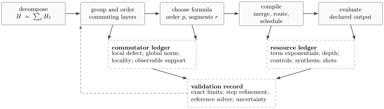
A product-formula result is fixed jointly by the decomposition, commuting groups and ordering, formula order and segment count, compiled realization, and requested output. The commutator, resource, and validation ledgers must remain attached to the same design.

Local Error, Global Error, and Cost

Suppose a one-step bound has been established for sufficiently small $|\tau|$:

$$\left\|S_p(\tau)-e^{\tau A}\right\| \leq C_{p+1}|\tau|^{p+1}.$$

Because both the exact and approximate steps are unitary, a telescoping sum gives

$$\begin{aligned} \left\|S_p(t/r)^r-e^{tA}\right\| &\leq r\left\|S_p(t/r)-e^{tA/r}\right\| \\ &\leq C_{p+1}\frac{|t|^{p+1}}{r^p}. \end{aligned}$$

It therefore suffices to choose

$$r \geq \left( \frac{C_{p+1}|t|^{p+1}}{\varepsilon_U} \right)^{1/p}.$$

If one step uses $m_p$ term exponentials after merging, the primitive count is approximately

$$N_{\exp}\simeq m_p r.$$

This pair of equations displays the real optimization problem. Increasing $p$ improves the power of $r$, but usually increases $m_p$, introduces larger coefficient magnitudes, and changes $C_{p+1}$. A fourth-order formula is not intrinsically cheaper than a second-order one.

A two-term first-order bound

For $H=H_A+H_B$, the unitary integral representation yields

$$\left\| e^{-iH_A\tau/\hbar} e^{-iH_B\tau/\hbar} -e^{-iH\tau/\hbar} \right\| \leq \frac{\tau^2}{2\hbar^2} \left\|[H_A,H_B]\right\|.$$

After $r$ segments,

$$\left\| S_1(t/r)^r-e^{-iHt/\hbar} \right\| \leq \frac{t^2}{2r\hbar^2} \left\|[H_A,H_B]\right\|.$$

The formula is exact at every step if $[H_A,H_B]=0$. A bound depending only on $\|H_A\|+\|H_B\|$ would miss this decisive structure.

A two-term second-order bound

For the $A$-sandwiched formula

$$S_2(\tau) = e^{-iH_A\tau/(2\hbar)} e^{-iH_B\tau/\hbar} e^{-iH_A\tau/(2\hbar)},$$

one convenient norm estimate is

$$\begin{aligned} \left\|S_2(\tau)-e^{-iH\tau/\hbar}\right\| \leq{}& \frac{|\tau|^3}{24\hbar^3} \left\|[H_A,[H_A,H_B]]\right\| \\ &+ \frac{|\tau|^3}{12\hbar^3} \left\|[H_B,[H_B,H_A]]\right\|. \end{aligned}$$

Interchanging which term is sandwiched interchanges the coefficients attached to the two nested commutators. Thus even the two possible Strang orderings can have meaningfully different error constants.

General commutator scaling

For a fixed order-$p$ formula, the leading coefficient can be bounded by a weighted sum of $(p+1)$-fold nested commutators. Schematically,

$$\alpha_{p+1} = \frac{1}{\hbar^{p+1}} \sum_{\boldsymbol\ell} c_{\boldsymbol\ell} \left\| [H_{\ell_{p+1}}, [H_{\ell_p},ldots,[H_{\ell_2},H_{\ell_1}]]\ldots] \right\|,$$

where the nonnegative weights $c_{\boldsymbol\ell}$ depend on the selected formula and ordering. A rigorous bound then has the form

$$\left\| S_p(t/r)^r-e^{-iHt/\hbar} \right\| \leq K_p\alpha_{p+1} \frac{|t|^{p+1}}{r^p},$$

within the theorem’s stated regime. The constant $K_p$ and the exact commutator sum must come from the chosen bound; the schematic definition is not a license to silently set them to one.

A norm-only estimate uses

$$\|[X,Y]\|\leq2\|X\|\,\|Y\|$$

repeatedly. It can replace structural zeros by a combinatorial number of nonzero terms and overestimate the required $r$ severely. Such a bound may be a valid certificate, but it should not be presented as a realistic resource prediction without comparison to tighter analysis or numerical evidence.

Decomposition, Grouping, and Ordering

The Hamiltonian split is part of the algorithm. Algebraically equivalent decompositions can have different commutator bounds and very different compiled costs.

Group commuting terms

If terms in a set $G_a$ commute, define

$$K_a=\sum_{\ell\in G_a}H_\ell.$$

Then

$$e^{-iK_a\tau/\hbar} = \prod_{\ell\in G_a} e^{-iH_\ell\tau/\hbar}$$

exactly, in any order within the group. Grouping can expose parallel layers and reduce the number of noncommuting blocks. It does not make the physical gates free: overlapping commuting Pauli rotations may still contend for the same qubits, and exponentiating a generic commuting sum can require a nontrivial basis change.

Order by both algebra and compilation

At finite $r$, changing the order changes the nested commutator coefficient. It can also change routing, basis-change cancellation, rotation merging, and parallel depth. A sensible ordering study therefore records at least two scores:

$$\text{algorithmic score} \sim \widehat\alpha_{p+1}, \qquad \text{compiled score} = (N_{2q},D_{2q},N_T,N_{\mathrm{route}},\ldots).$$

Minimizing one need not minimize the other. For electronic-structure Hamiltonians, term ordering has been observed to change finite-instance Trotter errors substantially even among formulas with identical formal order. The selected heuristic and any search budget should be reported, not hidden behind the final permutation.

Preserve exact cancellations

Before synthesizing individual rotations, simplify the symbolic product:

• merge adjacent exponentials of the same generator;
• commute disjoint operations into parallel layers;
• cancel inverse basis changes and parity networks when valid;
• retain parameter symbols until after merging equal rotations;
• distinguish an algebraic cancellation from one introduced only by an approximate compiler pass.

Compiling each segment independently and concatenating the results can miss boundary cancellations that are exact in $S_p(\tau)^r$.

Local Hamiltonians and Nearly Linear Scaling

Locality changes the system-size dependence because most formal nested commutators vanish. Consider an open one-dimensional chain

$$H=\sum_{j=1}^{n-1}h_{j,j+1}, \qquad \|h_{j,j+1}\|\leq J.$$

Split the bonds into odd and even layers,

$$H_{\mathrm o} = \sum_j h_{2j-1,2j}, \qquad H_{\mathrm e} = \sum_j h_{2j,2j+1}.$$

Terms commute within each layer because their supports are disjoint. A nested commutator of fixed depth has bounded spatial support, and only $O(n)$ of its translations are nonzero. For a fixed order $p$, a representative scaling is

$$\left\|S_p(t/r)^r-e^{-iHt/\hbar}\right\| = O\!\left( n\frac{(J|t|/\hbar)^{p+1}}{r^p} \right),$$

where the hidden constant depends on the formula, interaction range, and local geometry. It is enough to take

$$r = O\!\left[ \frac{J|t|}{\hbar} \left( \frac{nJ|t|}{\hbar\varepsilon_U} \right)^{1/p} \right].$$

Since each segment uses $O(n)$ local gates at fixed $p$, the gate count obeys

$$N_{\mathrm{gate}} = O\!\left[ n\frac{J|t|}{\hbar} \left( \frac{nJ|t|}{\hbar\varepsilon_U} \right)^{1/p} \right].$$

Choosing increasingly high even order while accounting for Suzuki’s stage growth gives nearly linear asymptotic scaling for finite-range lattice Hamiltonians, commonly summarized as $(nt)^{1+o(1)}$ in units with bounded local interaction strength and fixed accuracy conventions. That statement is not a guarantee that very high order wins at a finite problem size.

Higher-dimensional lattices

On a finite-range interaction graph, edge coloring partitions local terms into sets of disjoint interactions. For a hypercubic nearest-neighbor lattice in $D$ dimensions, a $2D$-color construction provides a constant number of commuting layers. Each layer contains $O(n)$ gates but can have constant ideal depth when all disjoint gates are natively executable in parallel.

Gate count and depth must therefore be stated separately. If a fixed-order step has $q_p=O(1)$ commuting-layer modules, then ideally

$$N_{2q}=O(nr q_p), \qquad D_{2q}=O(rq_p)$$

for an ideal bounded-degree architecture, before routing and control constraints. A device whose connectivity does not match the interaction graph can lose the depth advantage.

Local observables

Suppose the requested output is

$$\langle O(t)\rangle = \operatorname{Tr}\!\left[ \rho\,e^{iHt/\hbar}Oe^{-iHt/\hbar} \right]$$

for an observable supported on a fixed region. Under finite-range or suitably decaying interactions, only terms inside the observable’s effective light cone can influence it appreciably at finite time. A locality-aware product formula can omit operations outside a buffered causal region and use an error analysis tied directly to $O$.

For fixed time and local accuracy, this can remove the dependence on the total system size once the system is larger than the required light cone. The cost still grows with time, interaction range, desired precision, and the support of $O$. It also does not supply a full-unitary approximation for later use by an arbitrary algorithm.

Worked Example: Transverse-Field Ising Chain

For an open chain of $n$ qubits, take

$$H = H_{ZZ}+H_X,$$

with

$$H_{ZZ} = -J\sum_{j=1}^{n-1}Z_jZ_{j+1}, \qquad H_X = -h\sum_{j=1}^{n}X_j.$$

All terms commute within $H_{ZZ}$, and all terms commute within $H_X$. Consequently,

$$\begin{aligned} e^{-iH_{ZZ}\tau/\hbar} &= \prod_{j=1}^{n-1} e^{iJ\tau Z_jZ_{j+1}/\hbar}, \\ e^{-iH_X\tau/\hbar} &= \prod_{j=1}^{n} e^{ih\tau X_j/\hbar}. \end{aligned}$$

A second-order step is

$$S_2(\tau) = e^{-iH_{ZZ}\tau/(2\hbar)} e^{-iH_X\tau/\hbar} e^{-iH_{ZZ}\tau/(2\hbar)}.$$

The source of product-formula error is not the number of terms by itself, but their cross-commutator:

$$[H_X,H_{ZZ}] = -2ihJ \sum_{j=1}^{n-1} \left( Y_jZ_{j+1}+Z_jY_{j+1} \right).$$

The elementary norm bound

$$\|[H_X,H_{ZZ}]\| \leq 4|hJ|(n-1)$$

makes the extensive first-order scaling explicit, although it need not be tight. If either $h=0$ or $J=0$, the commutator vanishes and the split is exact.

Circuit anatomy

Define $R_Z(\phi)=e^{-i\phi Z/2}$. A nearest-neighbor interaction rotation can be synthesized as

$$e^{-i\theta Z_jZ_{j+1}} = \operatorname{CX}_{j,j+1} R_Z^{(j+1)}(2\theta) \operatorname{CX}_{j,j+1}.$$

Each $X$ rotation is a single-qubit operation. Although all $ZZ$ rotations commute, adjacent bonds share a qubit; on a conventional circuit scheduler they form odd- and even-bond sublayers. The $X$ rotations form one parallel layer.

Across $r$ symmetric steps, adjacent $ZZ$ half steps at segment boundaries merge. The symbolic circuit therefore contains

$$r n$$

$X$ rotations and

$$(r+1)(n-1)$$

$ZZ$ rotations, including the two half-angle boundary layers. A naive segment-by-segment count of $2r(n-1)$ $ZZ$ rotations misses this exact reduction.

The ideal second-order error scales as $r^{-2}$ at fixed $n$, $J$, $h$, and $t$. A practical study should verify that slope on small exactly solvable instances, then check the observable of interest as $r$ is doubled on the target workflow. Transverse-Field Ising Model owns the model’s phases and physical interpretation.

Pauli-String Exponentials

After a qubit encoding, many applications produce

$$H=\sum_{\ell=1}^{L}h_\ell P_\ell,$$

where each $P_\ell$ is a tensor product of Pauli operators. Since $P_\ell^2=I$,

$$e^{-i\theta P_\ell} = \cos\theta\,I-i\sin\theta\,P_\ell.$$

For a weight-$w$ string, a standard synthesis performs local basis changes, computes the parity onto one qubit, applies $R_Z(2\theta)$, uncomputes the parity, and reverses the basis changes. On all-to-all connectivity, a simple ladder uses $2(w-1)$ entangling gates. Hardware connectivity, native parity operations, ancilla availability, and neighboring strings can change that count substantially.

For the Hamiltonian coefficient $h_\ell$, the rotation parameter in one first-order segment is

$$\theta_\ell = \frac{h_\ell t}{r\hbar}.$$

The factor of two in the physical $R_Z$ angle follows from the convention $R_Z(\phi)=e^{-i\phi Z/2}$. Confusing $\theta_\ell$ with $\phi$ produces a factor-of-two simulation error, not a small synthesis error.

Controlled evolution

Phase estimation and some correlation-function protocols require controlled $\widetilde U_p(t;r)$, not merely the uncontrolled circuit. Every term exponential, frame change, routing operation, and inverse must then be controlled or replaced by an equivalent construction. A resource estimate for uncontrolled Trotter evolution cannot be reused unchanged.

Randomized Product Formulas

Deterministic formulas use a fixed ordering in every segment. A randomized formula may sample a permutation $\pi_s$ for segment $s$ and apply

$$S_{1,\pi_s}(\tau) = \prod_{j=1}^{L} e^{-iH_{\pi_s(j)}\tau/\hbar}.$$

Randomization can cancel coherent contributions in expectation and supports stronger error bounds in important regimes. It also changes the object being analyzed. Averaging over sampled circuits gives the channel

$$\mathcal E_\tau(\rho) = \mathbb E_\pi\!\left[ S_{1,\pi}(\tau)\rho S_{1,\pi}(\tau)^\dagger \right],$$

which is generally not the unitary channel generated by one “average circuit.” A theorem about expected channel error does not imply that every sampled trajectory has the same error. One must report whether permutations are sampled once, independently by segment, or independently by experimental shot, and how randomization variance enters the estimator.

Randomly permuting every term is also distinct from qDRIFT, which samples individual Hamiltonian terms with probabilities proportional to their coefficient magnitudes. The two methods have different channels, complexity parameters, and guarantees.

Time-Dependent Hamiltonians

For

$$H(s)=\sum_{\ell=1}^{L}H_\ell(s),$$

the target propagator is time ordered:

$$U(t,0) = \mathcal T \exp\!\left[ -\frac{i}{\hbar} \int_0^t H(s)\,ds \right].$$

There are now at least two discretization problems:

1. approximating the chronological variation of $H(s)$ within each interval;
2. splitting the noncommuting terms at the selected sample times.

A basic first-order step over $[t_j,t_j+\tau]$ is

$$\widetilde U_j = \prod_{\ell=L}^{1} \exp\!\left[ -\frac{i\tau}{\hbar}H_\ell(t_j) \right].$$

Its error contains time-sampling contributions involving temporal variation and splitting contributions involving commutators. Replacing $t_j$ by a midpoint can improve quadrature accuracy under smoothness assumptions, but it does not by itself create an arbitrary-order time-dependent Suzuki formula. Higher-order constructions require correctly placed evaluation times or explicit time-ordered exponentials.

Useful bounds depend on quantities such as

$$\int_0^t\|H(s)\|\,ds, \qquad \int_0^t\|\dot H(s)\|\,ds,$$

and time-separated commutators

$$[H_\ell(s),H_m(s')].$$

The sampling rule, smoothness assumptions, and oracle or control cost for evaluating $H_\ell(s)$ must be stated. When $H=H_0+\lambda H_1$ has separated energy scales and $H_0$ is cheaply implementable, an interaction-picture, time-dependent product formula can replace a bound governed by $\|H_0\|+\|\lambda H_1\|$ with one that exploits the small perturbation and transformed commutators. This improvement is structural, not a generic property of midpoint sampling.

Product Formulas and Phase Estimation

If phase estimation uses a finite-step product formula, it resolves eigenphases of the implemented unitary

$$S_p(\tau) = e^{-iH_{\mathrm{eff}}(\tau)\tau/\hbar},$$

for a branch-dependent effective Hamiltonian

$$H_{\mathrm{eff}}(\tau) = \frac{i\hbar}{\tau}\log S_p(\tau).$$

It does not directly return exact eigenvalues of $H$. For a symmetric order-$p$ formula, the effective-Hamiltonian correction begins at order $\tau^p$ under suitable spectral and branch conditions. Energy bias can be state dependent, and energy differences may exhibit cancellations not visible in a full-unitary norm bound.

If

$$\|S_p(\tau)^r-e^{-iHt/\hbar}\| \leq \varepsilon_U<2,$$

then paired eigenvalues on the unit circle have chordal displacement at most $\varepsilon_U$, corresponding locally to an eigenphase displacement bounded by

$$|\delta\phi| \leq 2\arcsin\!\left(\frac{\varepsilon_U}{2}\right).$$

Away from phase-wrap ambiguities, the corresponding energy scale is

$$|\delta E| \lesssim \frac{\hbar}{|t|} 2\arcsin\!\left(\frac{\varepsilon_U}{2}\right).$$

This is only the product-formula contribution. Finite phase-register resolution, eigenstate overlap, synthesis, controlled-circuit errors, and phase aliasing remain separate. Quantum Phase Estimation develops those parts of the contract.

Error and Resource Ledgers

A trustworthy simulation separates ideal algorithmic approximation from the implementation that realizes it. One useful decomposition is

$$\varepsilon_{\mathrm{total}} \leq \varepsilon_{\mathrm{model}} +\varepsilon_{\mathrm{enc}} +\varepsilon_{\mathrm{PF}} +\varepsilon_{\mathrm{synth}} +\varepsilon_{\mathrm{route}} +\varepsilon_{\mathrm{hw}} +\varepsilon_{\mathrm{stat}}.$$

The terms represent model reduction, finite encoding or truncation, product-formula approximation, gate synthesis, routing and compilation, hardware noise, and statistical estimation. This is a budgeting inequality, not a claim that all errors physically add with the same sign or coherence.

The matching resource record should include

$$\mathcal R = \left( n_{\mathrm{logical}}, r, p, N_{\exp}, N_{1q}, N_{2q}, D_{2q}, N_T, n_{\mathrm{anc}}, N_{\mathrm{shots}}, t_{\mathrm{wall}} \right).$$

Which entries matter depends on the regime. Near-term experiments often care about routed two-qubit depth and shots. Fault-tolerant studies often care about logical qubits, non-Clifford count and depth, magic-state throughput, and the cost of controlled evolution.

Choosing a finite segment count under noise

On an ideal computer, increasing $r$ reduces product-formula error. On a noisy device, a coarse diagnostic model may be

$$\varepsilon_{\mathrm{proxy}}(r) = \frac{A}{r^p}+Br,$$

where the first term represents algorithmic error and the second represents depth-proportional implementation error. Treating $r$ as continuous gives

$$r_* = \left(\frac{pA}{B}\right)^{1/(p+1)}.$$

This explains why “more Trotter steps” can worsen measured performance. The model is not universal: coherent gate errors, cancellation, drift, leakage, and mitigation can violate the linear term. It is a design diagnostic to be validated, not a substitute for device characterization.

Validation and Convergence

Formal order should be checked against the implemented workflow.

Exact small-instance benchmarks

For small Hilbert spaces, compute

$$\delta_U(r) = \min_{\phi\in\mathbb R} \left\| e^{i\phi}\widetilde U_p(t;r)-e^{-iHt/\hbar} \right\|.$$

The phase minimization is appropriate when the unitary is used only as an uncontrolled channel, because a global phase then has no operational effect. For controlled evolution or phase estimation, compare without that minimization: the relative phase between control branches is observable. Also compare state fidelity, conserved quantities, and the actual target observable. A commuting instance is a useful zero-error test but cannot measure convergence order.

Refinement studies

In the asymptotic regime,

$$\delta(r)=c r^{-p}+O(r^{-p-1})$$

for a generic order-$p$ formula. An observed order can be estimated from three successive refinements:

$$p_{\mathrm{obs}} = \log_2\!\left| \frac{Q(r)-Q(2r)}{Q(2r)-Q(4r)} \right|.$$

This estimate is meaningful only when the denominator is resolved and the same state preparation, compiler, measurement protocol, and noise treatment are used. Accidental cancellation can produce a temporarily higher slope.

If the leading model is credible, Richardson extrapolation gives

$$Q_{\mathrm{ext}} = \frac{2^pQ(2r)-Q(r)}{2^p-1}.$$

Extrapolation can reduce bias in an observable but does not prepare a more accurate quantum state. It can also amplify statistical uncertainty and fail when hardware noise changes with depth.

Structural checks

A good validation suite includes:

• exactness when all declared groups commute;
• unitarity of every ideal finite-step circuit;
• time-reversal symmetry for symmetric formulas;
• invariance under algebraically equivalent gate merging;
• convergence of the requested observable under $r\mapsto2r$;
• comparison against exact diagonalization, tensor networks, free limits, or perturbative results where available;
• separate ideal-circuit and noisy-device results;
• at least one benchmark outside the parameter point used to tune ordering.

Trotter Evolution Notebook gives a compact finite-dimensional workflow for measuring first- and second-order slopes.

Method Selection

Product formulas are especially attractive when

• term exponentials are native or compile compactly;
• the decomposition has sparse nested commutators or geometric locality;
• low ancilla count matters;
• a moderate accuracy is sufficient;
• the output is local and admits a light-cone reduction;
• symbolic cancellation and parallel scheduling reduce the realized depth.

They become less attractive when

• precision is so stringent that polynomial dependence on $1/\varepsilon$ dominates;
• the Hamiltonian has many strongly noncommuting terms with costly exponentials;
• controlled term evolution is much more expensive than block-encoded access;
• high-order negative coefficients are incompatible with the control model;
• a block encoding already supports qubitization with a favorable normalization;
• long-time full-unitary accuracy, rather than a restricted observable, is required.

The comparison must use the same Hamiltonian representation, output, accuracy, architecture, and fault-tolerance assumptions. An oracle-query bound for qubitization and a routed gate count for Trotterization are not commensurate resources.

Reporting Checklist

A product-formula simulation should report:

Item	Required information
target	Hamiltonian, units, total time, initial state, and requested output
decomposition	every $H_\ell$, coefficient convention, grouping, and term order
formula	explicit sequence or recursion, order $p$, coefficients, and segment count $r$
guarantee	norm or observable, tolerance, theorem assumptions, and bound used
implementation	synthesis of each exponential, controls, connectivity, routing, and cancellations
resources	primitive rotations, one- and two-qubit gates, depth, ancillas, shots, and fault-tolerant costs as applicable
uncertainty	product-formula, synthesis, hardware, statistical, and model contributions kept distinct
validation	exact limits, refinement data, reference solver, conserved quantities, and tested parameter range
randomization	sampling distribution, resampling schedule, seed policy, and variance contribution
provenance	software version, compiler settings, hardware calibration window, and reproducible circuit description

The explicit sequence matters. Two studies that both say “second-order Trotter” can use different splits, sandwich terms, segment boundaries, compilers, and observables, and therefore implement materially different algorithms.

Common Mistakes

• Treating $e^{A+B}=e^Ae^B$ as exact when $[A,B]\ne0$.
• Reporting formula order without its commutator coefficient or tested convergence regime.
• Using a one-step $O(\tau^{p+1})$ statement as though the fixed-time global error were also $O(r^{-(p+1)})$; it is generically $O(r^{-p})$.
• Replacing every nested commutator by a product of norms and presenting the resulting loose certificate as a realistic resource forecast.
• Counting term exponentials before merging symmetric segment boundaries.
• Assuming commuting rotations are simultaneously executable when they share hardware resources.
• Ignoring the negative coefficients and stage growth of higher-order Suzuki formulas.
• Calling a random term-sampling algorithm qDRIFT and a random permutation formula the same method.
• Combining time-sampling and operator-splitting error into one unnamed “Trotter error.”
• Increasing $r$ on noisy hardware without checking the depth-versus-bias tradeoff.
• Using an uncontrolled circuit cost for a phase-estimation protocol that requires controlled evolution.
• Validating only on a commuting split or on the parameter point used to tune the ordering.

Knowledge Status

The Trotter product limit, symmetric splitting, Suzuki recursion, and fixed-order convergence theory are established mathematics under their stated operator assumptions. Commutator-sensitive bounds and nearly linear lattice scaling are also rigorous results for specified Hamiltonian classes and metrics.

Finite-instance performance remains representation and implementation dependent. Ordering heuristics, empirical error estimators, compiler-aware formula search, observable-specific cancellation, and noise-aware segment selection are active areas of research. Improvements demonstrated for one Hamiltonian family, state sector, or device should not be generalized without a matched analysis.

References

1. H. F. Trotter, “On the Product of Semi-Groups of Operators,” Proceedings of the American Mathematical Society 10, 545–551 (1959), doi:10.2307/2033649.
2. G. Strang, “On the Construction and Comparison of Difference Schemes,” SIAM Journal on Numerical Analysis 5, 506–517 (1968), doi:10.1137/0705041.
3. M. Suzuki, “Generalized Trotter’s Formula and Systematic Approximants of Exponential Operators and Inner Derivations with Applications to Many-Body Problems,” Communications in Mathematical Physics 51, 183–190 (1976), doi:10.1007/BF01609348.
4. M. Suzuki, “Fractal Decomposition of Exponential Operators with Applications to Many-Body Theories and Monte Carlo Simulations,” Physics Letters A 146, 319–323 (1990), doi:10.1016/0375-9601(90)90962-N.
5. Q. Sheng, “Solving Linear Partial Differential Equations by Exponential Splitting,” IMA Journal of Numerical Analysis 9, 199–212 (1989), doi:10.1093/imanum/9.2.199.
6. D. W. Berry, G. Ahokas, R. Cleve, and B. C. Sanders, “Efficient Quantum Algorithms for Simulating Sparse Hamiltonians,” Communications in Mathematical Physics 270, 359–371 (2007), doi:10.1007/s00220-006-0150-x.
7. A. M. Childs, D. Maslov, Y. Nam, N. J. Ross, and Y. Su, “Toward the First Quantum Simulation with Quantum Speedup,” Proceedings of the National Academy of Sciences 115, 9456–9461 (2018), doi:10.1073/pnas.1801723115.
8. A. M. Childs, A. Ostrander, and Y. Su, “Faster Quantum Simulation by Randomization,” Quantum 3, 182 (2019), doi:10.22331/q-2019-09-02-182.
9. A. M. Childs and Y. Su, “Nearly Optimal Lattice Simulation by Product Formulas,” Physical Review Letters 123, 050503 (2019), doi:10.1103/PhysRevLett.123.050503.
10. A. M. Childs, Y. Su, M. C. Tran, N. Wiebe, and S. Zhu, “Theory of Trotter Error with Commutator Scaling,” Physical Review X 11, 011020 (2021), doi:10.1103/PhysRevX.11.011020.
11. R. Babbush, J. McClean, D. Wecker, A. Aspuru-Guzik, and N. Wiebe, “Chemical Basis of Trotter–Suzuki Errors in Quantum Chemistry Simulation,” Physical Review A 91, 022311 (2015), doi:10.1103/PhysRevA.91.022311.
12. D. Poulin, M. B. Hastings, D. Wecker, N. Wiebe, A. C. Doherty, and M. Troyer, “The Trotter Step Size Required for Accurate Quantum Simulation of Quantum Chemistry,” Quantum Information and Computation 15, 361–384 (2015), arXiv:1406.4920.
13. A. Tranter, P. J. Love, F. Mintert, and P. V. Coveney, “Ordering of Trotterization: Impact on Errors in Quantum Simulation of Electronic Structure,” Entropy 21, 1218 (2019), doi:10.3390/e21121218.
14. I. D. Kivlichan et al., “Improved Fault-Tolerant Quantum Simulation of Condensed-Phase Correlated Electrons via Trotterization,” Quantum 4, 296 (2020), doi:10.22331/q-2020-07-16-296.
15. J. Huyghebaert and H. De Raedt, “Product Formula Methods for Time-Dependent Schrödinger Problems,” Journal of Physics A: Mathematical and General 23, 5777–5793 (1990), doi:10.1088/0305-4470/23/24/019.
16. N. Wiebe, D. Berry, P. Høyer, and B. C. Sanders, “Higher Order Decompositions of Ordered Operator Exponentials,” Journal of Physics A: Mathematical and Theoretical 43, 065203 (2010), doi:10.1088/1751-8113/43/6/065203.
17. J. L. Bosse, A. M. Childs, C. Derby, F. M. Gambetta, A. Montanaro, and R. A. Santos, “Efficient and Practical Hamiltonian Simulation from Time-Dependent Product Formulas,” Nature Communications 16, 2931 (2025), doi:10.1038/s41467-025-57580-5.
18. E. Campbell, “Random Compiler for Fast Hamiltonian Simulation,” Physical Review Letters 123, 070503 (2019), doi:10.1103/PhysRevLett.123.070503.
19. S. Lloyd, “Universal Quantum Simulators,” Science 273, 1073–1078 (1996), doi:10.1126/science.273.5278.1073.
20. M. A. Nielsen and I. L. Chuang, Quantum Computation and Quantum Information, 10th anniversary ed., Cambridge University Press (2010).

Further Connections

• Hamiltonian Simulation compares product formulas with other access models and algorithm families.
• Digital Quantum Simulation places the product-formula circuit inside the full encoding, compilation, execution, and readout workflow.
• Qubitization and Quantum Signal Processing develops the principal block-encoding alternative, including its normalization, precision, oracle, and phase-synthesis costs.
• Trotter Product Formula gives the canonical operator derivation and convergence logic.
• Baker–Campbell–Hausdorff Formula explains how commutators enter short formal expansions.
• Circuit Optimization develops gate cancellation, commutation, layout-aware rewriting, and semantic verification.
• Resource Estimation Tools owns end-to-end logical and physical resource accounting.
• Algorithmic Benchmarking defines matched estimands, baselines, and uncertainty for algorithm comparisons.
• Simulation of Quantum Materials supplies periodic, Hubbard, and spin-model instances whose geometry, representation, observable, and precision determine whether product formulas are competitive.
• Quantum Chemistry Case Studies examines representation and resource choices in concrete molecular workflows.

Exercises

1. Derive the global order

Assume $S_p(\tau)$ and $e^{\tau A}$ are unitary and

$$\|S_p(\tau)-e^{\tau A}\| \leq C|\tau|^{p+1}.$$

Prove the fixed-time bound for $r$ equal segments.

Solution

Use the identity

$$X^r-Y^r = \sum_{j=0}^{r-1} X^{r-1-j}(X-Y)Y^j$$

with $X=S_p(t/r)$ and $Y=e^{tA/r}$. Unitary invariance and submultiplicativity give

$$\|X^r-Y^r\| \leq \sum_{j=0}^{r-1}\|X-Y\| \leq rC\left|\frac{t}{r}\right|^{p+1}.$$

Therefore

$$\|S_p(t/r)^r-e^{tA}\| \leq C\frac{|t|^{p+1}}{r^p}.$$

The loss of one power relative to the local defect comes from accumulating $r$ steps.

2. Compare the two Strang orderings

For $H=H_A+H_B$, suppose

$$X=\|[H_A,[H_A,H_B]]\|, \qquad Y=\|[H_B,[H_B,H_A]]\|.$$

Using the bound on this page, which term should be placed on the outside if $X\gg Y$?

Solution

For the $A$-sandwiched formula, the displayed coefficient is

$$\frac{X}{24}+\frac{Y}{12}.$$

For the $B$-sandwiched formula, the roles are interchanged:

$$\frac{Y}{24}+\frac{X}{12}.$$

If $X\gg Y$, placing $A$ on the outside gives the smaller bound because the large nested commutator receives coefficient $1/24$ rather than $1/12$. This comparison concerns one bound; compiled gate cost can still reverse the practical choice.

3. Count merged second-order factors

Show that $r$ repetitions of a reduced symmetric step with $L$ ordered terms contain $r(2L-2)+1$ term exponentials after merging only exact segment-boundary factors.

Solution

One reduced symmetric step contains $2L-1$ exponentials. At each of the $r-1$ boundaries, its final $e^{\tau A_1/2}$ is adjacent to the next step’s initial $e^{\tau A_1/2}$. They combine exactly into $e^{\tau A_1}$, removing one exponential from the count. Hence

$$r(2L-1)-(r-1) = r(2L-2)+1.$$

Additional reductions require more information about commutation and the compiled realization.

4. Ising-chain commutator

Derive

$$[H_X,H_{ZZ}] = -2ihJ\sum_{j=1}^{n-1} (Y_jZ_{j+1}+Z_jY_{j+1}).$$

Solution

Only an $X_k$ acting on one endpoint of $Z_jZ_{j+1}$ contributes. Using $[X,Z]=-2iY$,

$$[X_j,Z_jZ_{j+1}] = -2iY_jZ_{j+1},$$

and

$$[X_{j+1},Z_jZ_{j+1}] = -2iZ_jY_{j+1}.$$

The product of the two Hamiltonian coefficients is $(-h)(-J)=hJ$. Summing over bonds gives the result. Terms with $k\notin\{j,j+1\}$ commute.

5. Optimize a noisy proxy

Minimize

$$f(r)=Ar^{-p}+Br$$

for positive $A$, $B$, and continuous $r>0$. Explain how an integer segment count should be selected.

Solution

Differentiate:

$$f'(r)=-pAr^{-(p+1)}+B.$$

The stationary point is

$$r_*=\left(\frac{pA}{B}\right)^{1/(p+1)}.$$

Since

$$f''(r)=p(p+1)Ar^{-(p+2)}>0,$$

it is a minimum. In an actual circuit, evaluate the feasible integers near $r_*$ after compilation, because depth can change discontinuously through gate cancellation and routing. The proxy should then be checked against measured or characterized noise.

6. Observable error from unitary error

Prove that $\|U-V\|\leq\delta$ implies

$$\left| \operatorname{Tr}[O(U\rho U^\dagger-V\rho V^\dagger)] \right| \leq2\|O\|\delta.$$

Solution

Insert and subtract $V\rho U^\dagger$:

$$U\rho U^\dagger-V\rho V^\dagger = (U-V)\rho U^\dagger +V\rho(U^\dagger-V^\dagger).$$

Hölder’s inequality gives

$$|\operatorname{Tr}(OX)| \leq \|O\|\,\|X\|_1.$$

Using $\|AXB\|_1\leq\|A\|\|X\|_1\|B\|$, unitary norms equal to one, $\|\rho\|_1=1$, and $\|U^\dagger-V^\dagger\|=\|U-V\|$ gives two contributions bounded by $\|O\|\delta$.

7. Separate time sampling from splitting

Suppose $H(s)=A(s)+B(s)$ on one interval of width $\tau$. Identify two errors in the approximation

$$e^{-iA(t_j)\tau/\hbar}e^{-iB(t_j)\tau/\hbar}.$$

What limits make each contribution vanish?

Solution

First, replacing the time-dependent generator throughout the interval by its left-endpoint value produces a time-sampling error. It vanishes when $H(s)$ is constant on the interval and decreases under refinement when the required regularity bounds hold.

Second, splitting the frozen exponential $e^{-i(A(t_j)+B(t_j))\tau/\hbar}$ into two factors produces a noncommutativity error. It vanishes when $[A(t_j),B(t_j)]=0$. A constant Hamiltonian removes the first error but not necessarily the second; commuting pieces remove the second but do not make a time-varying left-endpoint rule exact.

8. Design a local-observable benchmark

You want $\langle Z_1(t)\rangle$ in a long nearest-neighbor spin chain. Describe a benchmark that can test whether a light-cone-truncated product-formula calculation is accurate without certifying the full unitary.

Solution

Choose increasing spatial buffers of radius $R$ around site $1$ and increasing segment counts $r$. For each pair $(R,r)$, estimate the same observable using the same initial reduced state and boundary prescription. Check convergence under both $R\mapsto R+\Delta R$ and $r\mapsto2r$. On sizes accessible to a trusted classical solver, compare the full time trace rather than one tuned time point. Also test a solvable parameter limit and monitor any conserved quantity supported in the simulated region.

This establishes evidence for the declared local observable and time window. It does not certify the action of the circuit on arbitrary inputs or observables outside the retained region.