Analog Quantum Simulation

Analog quantum simulation uses the continuously acting, engineered dynamics of one quantum system to reproduce selected states, observables, or processes of a target quantum model. Instead of decomposing a target evolution into a universal gate sequence, the experiment arranges physical degrees of freedom and controls so that its effective Hamiltonian or open-system generator belongs to the desired model family.

The word analog does not mean uncontrolled, classical, or merely qualitative. Modern analog simulators can have site-resolved preparation, programmable geometry, time-dependent fields, randomized measurements, and closed-loop calibration. What distinguishes them is that a many-body interaction acts as a native physical process rather than as a sequence of logically specified elementary gates. This often gives large system sizes and direct access to dynamics, at the cost of a restricted model family and no generic error-correction layer between the target and the apparatus.

This page is the canonical home for the analog correspondence problem: the map from target states and observables to laboratory degrees of freedom, the reduction from a microscopic laboratory model to an effective target Hamiltonian, time and energy rescaling, generator and leakage error, control manifolds, state preparation, readout, and quantitative validation. What Is Quantum Simulation? owns the general scientific simulation contract and the digital–analog–hybrid taxonomy. Digital Quantum Simulation owns the gate-based execution stack. Platform pages own the detailed atomic, ionic, photonic, and circuit physics, while the many-body volumes own the target models themselves.

The Operational Task

An analog-simulation claim should identify more than a Hamiltonian name. A useful task specification is

$$\mathfrak A = \left( \mathcal H_{\mathrm{tar}}, \Omega_{\mathrm{state}}, \Omega_{\mathrm{obs}}, \Theta, \mathcal T, \epsilon, \delta \right).$$

Here:

• $\mathcal H_{\mathrm{tar}}$ is the target Hilbert space;
• $\Omega_{\mathrm{state}}$ is the family of target inputs to be represented;
• $\Omega_{\mathrm{obs}}$ is the family of target observables to be estimated;
• $\Theta$ is the target parameter region;
• $\mathcal T$ is the set of target times or preparation protocols;
• $\epsilon$ is the promised accuracy for the reported quantities;
• $\delta$ is the allowed statistical failure probability.

Restricting the state and observable families is not a defect. It is often the reason a specialized simulator can be useful. A device may faithfully reproduce local spin correlations following a quench without representing every state in the target Hilbert space or permitting arbitrary global measurements. The restriction must, however, be stated before examining the result.

Let $\mathcal E_{\mathrm{s}}$ encode target states into the laboratory system, let $\mathcal T_\tau^{\boldsymbol\lambda}$ be the laboratory evolution at control setting $\boldsymbol\lambda$, and let $\mathcal E_{\mathrm{o}}(O)$ be the laboratory observable associated with $O$. If target parameters are related to controls by $\boldsymbol\theta=f(\boldsymbol\lambda)$ and target time is $t=\alpha\tau$, the operational prediction is

$$\widetilde\mu_O(t) = \operatorname{Tr} \left[ \mathcal E_{\mathrm{o}}(O) \, \mathcal T_{t/\alpha}^{\boldsymbol\lambda} \left( \mathcal E_{\mathrm{s}}(\rho) \right) \right].$$

The ideal target value is

$$\mu_O(t) = \operatorname{Tr} \left[ O\, \Phi_t^{\boldsymbol\theta}(\rho) \right].$$

An observable-specific analog guarantee can therefore be written

$$\sup_{\substack{ \rho\in\Omega_{\mathrm{state}}\\ O\in\Omega_{\mathrm{obs}}\\ \boldsymbol\theta\in\Theta,\, t\in\mathcal T }} \left| \widetilde\mu_O(t)-\mu_O(t) \right| \le \epsilon.$$

This form makes three facts explicit. The guarantee can be local rather than global, it applies only over a declared regime, and it includes preparation and measurement as well as evolution. A statement that a device “implements the Ising model” is incomplete until these domains and interfaces are given.

The Hamiltonian Correspondence

For closed-system simulation, the central reduction often takes the form

$$P H_{\mathrm{lab}}(\boldsymbol\lambda) P = \alpha(\boldsymbol\lambda) V H_{\mathrm{tar}} \left( \boldsymbol\theta(\boldsymbol\lambda) \right) V^\dagger + \beta(\boldsymbol\lambda)P + \Delta H(\boldsymbol\lambda).$$

The ingredients have distinct meanings:

Symbol	Role
$V$	isometric encoding from the target Hilbert space into the simulator
$P=VV^\dagger$	projector onto the intended encoded subspace
$\alpha$	conversion between target and laboratory energy scales
$\beta$	constant energy shift within the encoded subspace
$\Delta H$	in-subspace mismatch: omitted terms, disorder, drift, and calibration error
$Q=I-P$	leakage sector outside the intended description

The projected equation is not enough by itself. Couplings $QH_{\mathrm{lab}}P$ can move population out of the encoded space, and virtual excursions into $Q$ can modify the effective Hamiltonian even when the final leakage population is small. The model reduction should therefore state the spectral separation, coupling scale, truncation order, and regime over which $P$ remains meaningful.

Time and energy rescaling

Suppose for the moment that $\Delta H=0$ and leakage is absent. Because $PV=V$, one has

$$H_{\mathrm{lab}}V = \alpha V H_{\mathrm{tar}} + \beta V.$$

Expanding the exponential or using functional calculus gives

$$e^{-iH_{\mathrm{lab}}\tau/\hbar}V = e^{-i\beta\tau/\hbar} V e^{-iH_{\mathrm{tar}}t/\hbar}, \qquad t=\alpha\tau.$$

The $\beta$ term contributes a global phase to an encoded pure state and cancels from density-operator evolution. The scale $\alpha$ is operationally important: it converts laboratory coherence time into reachable target time, laboratory thermal energy $k_{\mathrm B}T_{\mathrm{lab}}$ into the target energy $k_{\mathrm B}T_{\mathrm{lab}}/\alpha$, and frequency uncertainty into target-parameter uncertainty. A dimensionless temperature still requires division by a target coupling or other target energy scale.

The same mapping must hold for observables. In the ideal encoded subspace,

$$P O_{\mathrm{lab}} P = V O_{\mathrm{tar}}V^\dagger + \Delta O.$$

A correct Hamiltonian with an uncalibrated detector does not yield a correct target observable. Conversely, a detector may access a useful target observable even when it cannot reconstruct the full state.

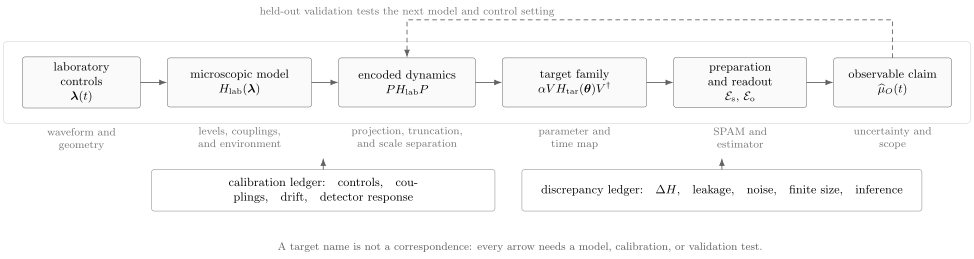
An analog simulator is an experimentally supported chain of reductions. Controls $\boldsymbol\lambda$ determine a microscopic laboratory model, projection and scale separation produce $H_{\mathrm{eff}}$, and a parameter map identifies the target family $H_{\mathrm{tar}}(\boldsymbol\theta)$. Preparation and readout complete the observable claim. Calibration constrains the map; held-out validation tests whether its discrepancy ledger is adequate.

Effective Hamiltonians are conditional

Many analog mappings are not exact microscopic identities. They are low-energy, rotating-frame, high-frequency, dispersive, or adiabatically eliminated descriptions. Schematically, if $H_0$ separates $P$ and $Q$ by a gap $\Delta_{\mathrm{sep}}$ and $W$ couples them, perturbative elimination produces

$$H_{\mathrm{eff}} = P(H_0+W)P - PWQ \left( QH_0Q-E \right)^{-1} QWP + \cdots.$$

The correction is typically of order $\lVert W\rVert^2/\Delta_{\mathrm{sep}}$, but coefficients and signs depend on the convention and spectrum. Schrieffer–Wolff Transformation owns the systematic block-diagonalization. Adiabatic Elimination and Average Hamiltonian Theory own two other common reductions.

Calling a Hamiltonian “effective” does not authorize dropping every inconvenient term. A mature reduction lists:

1. the retained subspace and basis;
2. the dimensionless expansion parameters;
3. the first omitted coherent terms;
4. the leakage channels;
5. the time window before secular corrections accumulate;
6. independent measurements that test the reduction.

Native Dynamics and Restricted Programmability

A convenient control model is

$$H_{\mathrm{lab}} \left( \boldsymbol\lambda,t \right) = H_0 + \sum_{a=1}^{m} u_a(\boldsymbol\lambda,t)H_a + H_{\mathrm{parasitic}} \left( \boldsymbol\lambda,t \right).$$

The drift $H_0$ and control generators $H_a$ define a physically reachable family. Geometry, laser frequency, magnetic field, interaction dressing, coupler bias, and trap depth may tune that family. They rarely tune every coefficient independently. One optical intensity can change a desired coupling, a light shift, and a scattering rate together; one geometric move can change several pair interactions at once.

An analog device is programmable when controls select a meaningful family of models, schedules, states, or observables. The term does not imply gate-model universality or arbitrary $k$-local Hamiltonian synthesis. Reports should distinguish:

• fixed: one Hamiltonian with a small number of global settings;
• tunable: continuous control of several global parameters;
• reconfigurable: geometry or coupling graph can be changed between runs;
• locally programmable: site- or bond-dependent parameters can be set;
• time programmable: ramps, quenches, Floquet drives, or feedback are available;
• universal: an explicit construction approximates a broad computational or Hamiltonian class with controlled resources.

These capabilities form a hierarchy only after accuracy and scaling are included. A nominally local control is not useful if its crosstalk grows unacceptably with system size. A universal construction based on exponentially large interaction strengths or exponentially precise controls is not a scalable simulator.

Dimensionless coordinates matter

Phase structure and dynamics usually depend on ratios such as

$$\frac{U}{J}, \qquad \frac{h}{J}, \qquad \frac{k_{\mathrm B}T}{J}, \qquad \frac{\gamma}{J/\hbar}, \qquad \frac{tJ}{\hbar},$$

not on a coupling in hertz by itself. Reporting dimensionless coordinates exposes whether a parameter scan changes only the intended target coordinate. For example, increasing lattice depth can simultaneously reduce tunnelling, change interaction matrix elements, alter heating, and modify adiabatic loading. The calibrated path through parameter space is then curved rather than a one-parameter line.

State Preparation

Analog evolution begins from a physical state, not from a symbolic ket. Common preparation routes include:

Route	Intended state	Principal difficulty
product initialization and quench	simple nonequilibrium input	SPAM bias and uncertain quench origin
adiabatic or quasi-adiabatic ramp	ground state connected to an easy state	small gaps, diabatic defects, heating
cooling and equilibration	thermal or low-energy ensemble	thermometry and equilibration evidence
dissipative preparation	steady state or dark state	generator identification and uniqueness
postselection	constrained or fixed-number sector	acceptance bias and resource accounting
local injection	excitation or response probe	pulse shape, spectral selectivity, back-action

For an interpolation $H(s)$ executed over total laboratory time $T$, a standard adiabatic diagnostic compares matrix elements of $\partial_s H$ with squared gaps:

$$\max_{\substack{s\in[0,1]\\m\ne 0}} \frac{ \hbar \left| \langle m(s)| \partial_s H(s) |0(s)\rangle \right| }{ T \left| E_m(s)-E_0(s) \right|^2 } \ll 1.$$

This is a useful scale estimate, not a universal certificate. Degeneracies, many-body gap closing, nonsmooth schedules, finite temperature, and open dynamics require more careful statements. Experimental evidence may combine forward-and-reverse ramps, defect scaling, energy estimates, local thermometry, symmetry checks, and agreement with solvable sizes.

A ground-state simulator does not become a finite-temperature simulator by failing to cool. Likewise, a finite-temperature experiment is not defective when the target question explicitly concerns a Gibbs ensemble and the temperature is estimated with uncertainty.

Evolution Protocols

Analog simulation includes more than passive evolution under one static Hamiltonian.

Quenches

A sudden parameter change prepares a simple state under one Hamiltonian and evolves it under another. Quenches probe transport, correlation spreading, prethermalization, relaxation, confinement, and dynamical phase structure. The switching time must be short relative to target dynamics but slow enough to avoid unmodeled levels when those levels are outside the target.

Ramps and anneals

Slow schedules aim to follow instantaneous low-energy states. Their outcome depends on the minimum gap, matrix elements, noise spectrum, schedule shape, and initial ensemble. An observed low energy does not by itself establish ground-state fidelity, especially when many states have similar energy.

Adiabatic Quantum Computation owns the ideal finite-dimensional closed-system computation-path contract and its circuit-equivalence ledger. This page retains target-to-device Hamiltonian correspondence, calibration, initial ensembles, leakage, noise, observables, and validation; a mathematical AQC path is not evidence that a laboratory ramp realizes it.

Quantum Annealing owns the complementary device-agnostic process record: driver–problem schedule, declared closed or reduced-open dynamics, endpoint samples, freeze-out hypothesis, decoder, and annealing-specific resources. That record does not establish the target-to-device correspondence retained here.

Periodic driving

Floquet protocols use periodic controls to generate an effective stroboscopic Hamiltonian. The drive frequency, micromotion, prethermal window, and heating rate are part of the simulation specification. A Floquet Hamiltonian is not a static Hamiltonian valid at arbitrary observation times.

Engineered dissipation

Reservoirs can cool, stabilize constraints, prepare steady states, or realize an open-system target. Uncontrolled decoherence becomes a target process only when its operators, rates, correlations, and domain match the desired generator. Lindblad–GKSL Equation owns the Markovian formalism and its assumptions.

How Hamiltonian Error Reaches an Observable

Let

$$H_{\mathrm{act}} = H_{\mathrm{tar}} + \Delta H$$

after encoding and unit conversion, and write

$$U(t)=e^{-iH_{\mathrm{tar}}t/\hbar}, \qquad \widetilde U(t)=e^{-iH_{\mathrm{act}}t/\hbar}.$$

Duhamel’s identity gives

$$\widetilde U(t)-U(t) = -\frac{i}{\hbar} \int_0^t \widetilde U(t-s) \Delta H U(s) \, ds.$$

Unitary invariance and submultiplicativity of the operator norm imply

$$\left\| \widetilde U(t)-U(t) \right\| \le \frac{|t|}{\hbar} \left\| \Delta H \right\|.$$

For an initial density operator $\rho$ and bounded observable $O$,

$$\begin{aligned} \left| \widetilde\mu_O(t)-\mu_O(t) \right| &= \left| \operatorname{Tr} \left[ O \left( \widetilde U\rho\widetilde U^\dagger - U\rho U^\dagger \right) \right] \right| \\ &\le 2 \left\|O\right\|_\infty \left\| \widetilde U(t)-U(t) \right\| \\ &\le \frac{2|t|}{\hbar} \left\|O\right\|_\infty \left\|\Delta H\right\|. \end{aligned}$$

This bound explains why a small generator mismatch can accumulate over time. It is also often pessimistic. For an extensive many-body Hamiltonian, $\lVert\Delta H\rVert$ can grow with system size even when the observable is local. Locality, Lieb–Robinson bounds, perturbative response, measured susceptibilities, or direct short-time tests can give sharper observable-specific estimates. The Lieb–Robinson Bound supplies the relevant locality structure.

Calibration uncertainty

Suppose a reported observable is modeled as $\mu(\boldsymbol\theta)$ and calibrated parameters have covariance matrix $\Sigma_\theta$. Linear uncertainty propagation gives

$$\operatorname{Var}_{\mathrm{cal}}(\mu) \approx \nabla_{\boldsymbol\theta}\mu^{\mathsf T} \Sigma_\theta \nabla_{\boldsymbol\theta}\mu.$$

Correlations matter. If one laser intensity shifts two couplings together, adding independent parameter error bars in quadrature is wrong. Near a critical point or resonance, the linear approximation may fail because susceptibilities are large or the response is nonlinear. Parameter ensembles, bootstrap propagation, or posterior predictive distributions are then preferable.

Leakage is not an in-subspace perturbation

Define the leakage probability at time $t$ by

$$p_{\mathrm{leak}}(t) = \operatorname{Tr} \left[ Q\widetilde\rho(t) \right].$$

Postselecting the $P$ sector changes the estimand. The conditional state

$$\rho_P(t) = \frac{ P\widetilde\rho(t)P }{ 1-p_{\mathrm{leak}}(t) }$$

can have accurate conditional observables even while the unconditional experiment has substantial failure probability. Both the conditional result and acceptance rate should be reported, along with whether leakage is detected without disturbing retained runs.

Error Classification

The same physical effect can be signal or error depending on the target.

Effect	Target feature when	Simulation error when
finite temperature	the target specifies a thermal ensemble	a ground-state claim silently uses a warm state
disorder	the disorder realization or ensemble is prescribed	uncontrolled inhomogeneity changes the intended clean model
dissipation	jump operators and rates define the target	decoherence is unmodeled or incorrectly correlated
long-range interaction	the target includes the calibrated tail	a nearest-neighbor model is claimed without bounding the tail
finite size and boundary	the finite geometry is the target	thermodynamic conclusions ignore size and edge effects
postselection	the conditional task is declared	discarded runs and resource cost are hidden
Floquet micromotion	observables are defined at physical times	only a stroboscopic effective model is reported as exact

This classification should be made at the level of the scientific question, not by labeling some hardware effects “good” and others “bad.” A noisy device does not automatically simulate open physics, and a long-range device does not automatically simulate a nearest-neighbor model.

Measurement and Inference

Analog simulators return detector records. The inference chain may include state-dependent fluorescence, atom or photon loss, parity projection, finite-resolution imaging, basis rotations, thresholding, and symmetry postselection.

For a discrete readout with ideal probabilities $\boldsymbol p$ and calibrated confusion matrix $M$, the observed distribution is

$$\boldsymbol q = M\boldsymbol p.$$

Inverting $M$ can remove bias under the model, but it amplifies variance when $M$ is ill-conditioned and can produce unphysical estimates at finite sample size. Regularization or constrained likelihood methods introduce their own bias. The raw counts, calibration data, estimator, and propagated uncertainty belong in the evidence record.

The useful output is usually modest:

• local densities or spin populations;
• one- and two-point correlation functions;
• structure factors and susceptibilities;
• full counting statistics in an accessible basis;
• response functions after a calibrated perturbation;
• subsystem entropies or overlaps from randomized measurements;
• energy estimates from a known decomposition;
• phase-boundary or scaling estimates with finite-size qualifications.

State tomography is neither necessary nor generally scalable. Measuring more observables does not automatically produce stronger evidence if they are all derived from the same untested calibration model.

Worked Example: A Rydberg Array as an Ising Simulator

Consider two internal states per atom: a ground state $|g\rangle$ and a Rydberg state $|r\rangle$. Choose Pauli conventions

$$Z_i|r_i\rangle=|r_i\rangle, \qquad Z_i|g_i\rangle=-|g_i\rangle, \qquad n_i=|r_i\rangle\langle r_i| = \frac{I+Z_i}{2}.$$

In a rotating-frame and rotating-wave description, a standard laboratory Hamiltonian is

$$H_{\mathrm{Ry}} = \sum_i \left( \frac{\hbar\Omega_i}{2}X_i - \hbar\Delta_i n_i \right) + \sum_{i<j} V_{ij}n_in_j.$$

For van der Waals interactions away from resonances,

$$V_{ij} \approx \frac{C_6}{R_{ij}^6},$$

with a sign and angular dependence set by the chosen states and geometry. The platform-specific interaction calculation and blockade approximations belong on Rydberg Atoms and Rydberg Blockade.

Exact spin expansion within the two-level model

Using

$$n_in_j = \frac{1}{4} \left( I+Z_i+Z_j+Z_iZ_j \right),$$

the Hamiltonian becomes

$$H_{\mathrm{Ry}} = C I + \sum_i \left( \frac{\hbar\Omega_i}{2}X_i + h_i^z Z_i \right) + \sum_{i<j} \frac{V_{ij}}{4}Z_iZ_j,$$

where

$$C = -\frac{\hbar}{2} \sum_i\Delta_i + \frac{1}{4} \sum_{i<j}V_{ij},$$

and

$$h_i^z = -\frac{\hbar\Delta_i}{2} + \frac{1}{4} \sum_{j\ne i}V_{ij}.$$

The interaction therefore produces both Ising couplings and site-dependent longitudinal fields. For a desired zero longitudinal field, the detuning must satisfy

$$\hbar\Delta_i = \frac{1}{2} \sum_{j\ne i}V_{ij}.$$

A single global detuning cancels this field only when the interaction sum is site independent. Edges, vacancies, geometry errors, and anisotropic interactions spoil that simplification. This is a direct example of why the control-to-model map must include geometry and the realized occupancy pattern.

Long-range tails define the actual target

Suppose the intended interpretation retains only a nearest-neighbor interaction $V_1$. The omitted coherent term is

$$\Delta H_{\mathrm{tail}} = \frac{1}{4} \sum_{\substack{i<j\\|i-j|>1}} V_{ij}Z_iZ_j + \text{associated longitudinal fields}.$$

A worst-case bound is

$$\left\| \Delta H_{\mathrm{tail}} \right\| \le \frac{1}{4} \sum_{\substack{i<j\\|i-j|>1}} \left|V_{ij}\right| + \left\| \Delta H_z \right\|.$$

For an infinite one-dimensional chain with $V_r=V_1/r^6$, the interaction energy per site from distances beyond nearest neighbors, relative to the nearest-neighbor contribution, is

$$\sum_{r=2}^{\infty}\frac{1}{r^6} = \zeta(6)-1 \approx 0.01734.$$

That number is small but not universally negligible. It can shift phase boundaries, lift degeneracies, alter constrained dynamics, or matter at long times. The scientifically clean alternatives are to include the calibrated tail in the target, demonstrate that the chosen observable is insensitive to it, or carry its effect as model discrepancy.

The blockade limit is another effective model

When nearest-neighbor excitation pairs cost an energy much larger than the drive and detuning scales, the dynamics can be projected into the no-adjacent- excitation subspace. The leading constrained Hamiltonian has the form

$$H_{\mathrm{PXP}} \approx \frac{\hbar\Omega}{2} \sum_i P_{i-1}X_iP_{i+1} - \hbar\Delta \sum_i n_i,$$

where $P_i=I-n_i$ projects site $i$ onto $|g_i\rangle$. Finite blockade, longer-range interactions, Rydberg decay, Doppler shifts, and preparation defects remain corrections. “PXP simulator” therefore names an effective regime, not an exact identity of the microscopic apparatus.

What a quantitative run should report

For this example, a credible record includes:

1. realized atom coordinates and vacancies for every accepted run;
2. calibrated $\Omega_i$, $\Delta_i$, and interaction model $V_{ij}$;
3. uncertainty and drift of those parameters;
4. preparation error and temperature or motional distribution where relevant;
5. ramp or quench waveform and timing;
6. loss, leakage, and readout confusion;
7. raw or minimally processed bitstrings;
8. the exact target Hamiltonian used in theory comparisons;
9. checks in small sizes, short times, symmetries, or solvable limits;
10. sensitivity of the reported observable to omitted terms.

Platform Families

Analog simulation is a method, not a single hardware architecture.

Platform	Native degrees of freedom and controls	Common target families	Characteristic model risk
optical lattices and quantum gases	atomic motion, internal states, lattice depth, scattering length, geometry	Bose–Hubbard, Fermi–Hubbard, spin, gauge, and continuum models	multiband terms, trap envelope, thermometry, loss, heating
neutral-atom and Rydberg arrays	two-level atoms, geometry, drive, detuning, pair interactions	Ising, XY, constrained, dimer, and optimization models	interaction tails, vacancies, decay, Doppler shifts, edge fields
trapped ions	internal spins, collective phonons, optical forces, mode shaping	long-range Ising and XY models, spin–boson dynamics	residual spin–motion entanglement, mode drift, interaction-matrix mismatch
superconducting circuits	qubits, resonators, tunable couplers, microwave drives	spin lattices, Bose–Hubbard variants, synthetic gauge and driven models	frequency disorder, crosstalk, photon loss, higher levels
polar molecules and magnetic atoms	rotational or spin states, dipolar interactions, external fields	long-range spin and lattice models	loss, tensor interactions, state-dependent trapping
photonic and polaritonic arrays	modes, hopping, drive, dissipation, nonlinearities	bosonic transport, synthetic dimensions, driven–dissipative matter	preparation and loss are inseparable from steady-state interpretation

Optical Lattices, Trapped-Ion Control, Neutral-Atom and Rydberg Qubits, and Superconducting Qubits give the platform-specific control and error physics. Lattice Models Overview and its linked model pages define the target Hamiltonians and observables.

Verification and Validation

Verification asks whether the apparatus implements the declared target task. Validation asks whether that target model answers the intended physical question. Verification of Quantum Simulation compares these protocols in depth; the essential analog workflow is given here.

A layered evidence ladder

1. Component calibration: characterize controls, couplings, detector response, loss, and drift independently where possible.
2. Generator checks: infer or constrain effective Hamiltonian and dissipative terms from dynamics, spectroscopy, response, or conservation laws.
3. Solvable overlap: compare with exact diagonalization, free limits, tensor networks, Monte Carlo without a sign problem, or perturbation theory where those methods are reliable.
4. Convergence and sensitivity: vary size, boundary, preparation, evolution time, interaction cutoff, and analysis assumptions.
5. Held-out prediction: calibrate on one set of states, times, or observables and predict another set without refitting.
6. Independent reproduction: compare platforms, implementations, observables, or laboratories with distinct systematic errors.
7. Frontier inference: report only the observable and regime supported by the preceding layers, with uncertainty and classical baselines.

Agreement in the calibration set is not yet prediction. A sufficiently flexible model can absorb error into fitted parameters. Held-out times, observables, initial states, or geometries test whether the inferred generator transfers beyond the data that selected it.

Hamiltonian learning

For a structured ansatz

$$H(\boldsymbol\theta) = \sum_{a=1}^{m}\theta_a H_a,$$

Hamiltonian learning estimates $\boldsymbol\theta$ from measured dynamics, steady states, response, or conserved quantities. It can expose coherent terms that component calibration misses. Its conclusion is conditional on the ansatz, identifiability, data range, SPAM model, and statistical uncertainty. A small residual within a misspecified ansatz does not prove that unmodeled operators are absent.

As of August 2026, bounded-error generator learning is an active research direction, not yet a platform-independent routine. Recent work combines Hamiltonian and Lindbladian learning with propagation of inferred generator uncertainty to many-body observables. Demonstrations can provide quantitative bounds under their stated ansatz, data, and open-system assumptions; they do not remove the need to test model misspecification, identifiability, and scaling beyond the demonstrated platform.

Cross-platform comparison

Independent simulators can compare local observables, probability distributions, or state overlaps inferred from randomized measurements. Agreement becomes stronger evidence when the platforms have different microscopic errors. It still does not prove correctness if both implement the same mistaken target map or share the same analysis assumptions.

Why extrapolation is difficult

Classical comparison often stops where the analog simulator becomes most interesting. Trust in that frontier regime must be earned by overlap: calibrated generators, size and time trends, conservation laws, solvable limits, alternative observables, and reproducible data. A single qualitative match at small size does not validate arbitrary larger systems or later times.

Resource Accounting

Analog hardware replaces a gate ledger with a different resource ledger:

Resource	What to report
physical size	sites, occupied sites, active modes, defects, accepted configurations
control complexity	independent global, local, geometric, and time-dependent controls
physical scale	coupling strengths, gaps, temperatures, dissipation rates, laboratory time
preparation	cooling, rearrangement, ramps, rejected runs, duty cycle
measurement	settings, destructive repetitions, detector efficiency, sample count
calibration	parameter count, cadence, data volume, classical fitting
stability	drift window, recalibration triggers, run ordering
classical work	model reduction, parameter inference, observable estimation, baselines
validation	held-out data, solvable regimes, independent checks

Continuous evolution is not free. Laboratory duration, coherence, cooling, loading, calibration, postselection, and repeated destructive measurement can dominate wall-clock cost. Likewise, “no gates” does not mean “no compilation”: geometry design, waveform optimization, parameter inversion, and schedule construction are forms of compilation into physical controls.

Analog, Digital, and Hybrid Boundaries

Question	Analog simulation	Digital simulation
What is programmed?	a physical Hamiltonian, channel, geometry, or control schedule	a logical circuit or algorithm
How does evolution occur?	native continuous many-body dynamics	discrete compiled operations
Typical approximation knob	detuning, scale separation, protection, truncation, or control precision	step count, polynomial degree, synthesis precision, or code distance
Flexibility	restricted but often physically natural family	broad under a universal gate and access model
Typical dominant risk	target–device mismatch and uncorrected physical noise	algorithmic overhead plus gate and logical error
Verification focus	generator, preparation, observable map, and held-out behavior	circuit implementation, logical error, and algorithmic approximation

The boundary is functional rather than cosmetic. Piecewise control does not make a protocol digital if each segment uses an uncompiled many-body interaction as its primitive. Conversely, a device built from analog pulses can implement digital gates when those pulses realize a calibrated discrete instruction set.

Digital–analog protocols compose native interaction blocks with discrete operations. Variational protocols use measured quantum states inside a classical feedback loop. Hybrid Quantum Simulation owns those architectures, including block-composition error, projected dynamics, self-consistent embedding, and feedback stability. What Is Quantum Simulation? provides the broader canonical taxonomy.

Claims About Quantum Advantage

Analog simulation can be scientifically useful before any complexity advantage is established. It can realize clean model experiments, reveal unexpected observables, test approximations, and guide theory in regimes where classical methods remain available.

A claim of advantage requires a sharper comparison:

1. define the input family and output quantity;
2. state accuracy and confidence;
3. count preparation, calibration, rejected runs, sampling, and classical inference;
4. compare with the best applicable classical methods for the same task;
5. justify correctness where full classical calculation is unavailable;
6. distinguish a hardware-scale milestone from a useful scientific result.

An exponentially large Hilbert space, a Monte Carlo sign problem, or failure of one tensor-network calculation is not by itself a proof. Classical tractability depends on model structure, dimension, entanglement, observable, time, and requested precision. Verification of Quantum Advantage owns the broader claim standard.

Common Mistakes

Treating the nominal Hamiltonian as the measured Hamiltonian

Control settings enter through a calibrated physical model. Interaction tails, inhomogeneity, higher levels, and correlated drift remain unless measured or bounded.

Assuming analog means exact

A native interaction removes one source of gate decomposition error. It does not remove model reduction, state preparation, noise, leakage, readout, or finite-sampling error.

Calling every tunable device universal

Programmability over a useful parameter family is valuable. Universality is a separate statement requiring an explicit simulation construction and scalable resource bounds.

Ignoring the observable map

Matching spectra or Hamiltonian coefficients does not guarantee that a detector measures the target quantity. Basis rotations, finite resolution, loss, and selection rules must be included.

Hiding postselection

A clean conditional result can coexist with a poor unconditional success rate. Report acceptance, the reason for rejection, and the resources spent on discarded runs.

Turning hardware noise into target physics by renaming it

Open-system simulation requires a declared generator and regime. Unknown decoherence is an uncertainty, not an engineered bath.

Fitting and validating on the same records

Agreement after parameter fitting checks consistency, not predictive power. Reserve held-out states, observables, times, or parameter points.

Extrapolating a local check into a global guarantee

Accurate densities at short time do not certify global fidelity, long-time dynamics, or all correlation functions. State the metric that was actually tested.

Reporting Checklist

Before interpreting an analog-simulation result, ask:

• What target state, parameter region, time window, and observables are claimed?
• What is the encoding $V$, and what physical subspace defines $P$?
• Which microscopic reduction produces the effective Hamiltonian?
• What are $\alpha$, $\beta$, $\Delta H$, and the leading leakage channels?
• Which controls are independent, and which target parameters are correlated?
• How were the initial state and detector response characterized?
• Is temperature, disorder, dissipation, or long-range coupling signal or error?
• Were uncertainty and drift propagated to the final observable?
• Which data calibrated the model, and which data were held out?
• What classical and cross-platform checks overlap the claimed regime?
• Are raw records, calibrations, exclusions, and analysis code available?
• Does the conclusion match the tested observable rather than a stronger unmeasured claim?

Key Results

For quick reference:

$$P H_{\mathrm{lab}}P = \alpha V H_{\mathrm{tar}}V^\dagger + \beta P + \Delta H$$

separates target dynamics, energy and time conversion, in-subspace mismatch, and the encoded subspace.

$$t_{\mathrm{tar}} = \alpha\tau_{\mathrm{lab}}$$

is the target-to-laboratory time conversion when $\alpha$ multiplies the target Hamiltonian in laboratory energy units.

$$\left\| \widetilde U(t)-U(t) \right\| \le \frac{|t|}{\hbar} \left\| \Delta H \right\|$$

is the basic bounded-Hamiltonian perturbation estimate.

$$\operatorname{Var}_{\mathrm{cal}}(\mu) \approx \nabla\mu^{\mathsf T} \Sigma_\theta \nabla\mu$$

propagates small correlated calibration uncertainty to an observable.

Further Connections

• What Is Quantum Simulation? defines the common simulation contract and evidence language.
• Digital Quantum Simulation develops the contrasting gate-based workflow and algorithmic error controls.
• Simulation of Quantum Materials places native Hubbard, spin, and bosonic realizations inside the broader material-model, finite-size, observable, and validation workflow.
• Device Characterization develops estimands, SPAM separation, drift, and characterization protocols.
• Reporting Standards gives the reproducibility record for hardware and application claims.
• Ultracold-Atom Quantum Simulation maintains the dated evidence ledger for optical-lattice and quantum-gas results.
• Optical Lattices derives the continuum-to-band and Hubbard-parameter reductions.
• Neutral-Atom and Rydberg Qubits and Trapped-Ion Qubits describe architecture-level capabilities and limitations.
• Quantum Channels and Noise supplies channel metrics for open and imperfect dynamics.
• Claims, Hype, and Evidence Standards separates demonstrated capability from extrapolation.

References

1. R. P. Feynman, “Simulating physics with computers,” International Journal of Theoretical Physics 21, 467–488 (1982), doi:10.1007/BF02650179.
2. I. Buluta and F. Nori, “Quantum simulators,” Science 326, 108–111 (2009), doi:10.1126/science.1177838.
3. J. I. Cirac and P. Zoller, “Goals and opportunities in quantum simulation,” Nature Physics 8, 264–266 (2012), doi:10.1038/nphys2275.
4. P. Hauke, F. M. Cucchietti, L. Tagliacozzo, I. Deutsch, and M. Lewenstein, “Can one trust quantum simulators?” Reports on Progress in Physics 75, 082401 (2012), doi:10.1088/0034-4885/75/8/082401.
5. I. M. Georgescu, S. Ashhab, and F. Nori, “Quantum simulation,” Reviews of Modern Physics 86, 153–185 (2014), doi:10.1103/RevModPhys.86.153.
6. I. Bloch, J. Dalibard, and S. Nascimbène, “Quantum simulations with ultracold quantum gases,” Nature Physics 8, 267–276 (2012), doi:10.1038/nphys2259.
7. C. Gross and I. Bloch, “Quantum simulations with ultracold atoms in optical lattices,” Science 357, 995–1001 (2017), doi:10.1126/science.aal3837.
8. C. Monroe et al., “Programmable quantum simulations of spin systems with trapped ions,” Reviews of Modern Physics 93, 025001 (2021), doi:10.1103/RevModPhys.93.025001.
9. A. Browaeys and T. Lahaye, “Many-body physics with individually controlled Rydberg atoms,” Nature Physics 16, 132–142 (2020), doi:10.1038/s41567-019-0733-z.
10. F. Schäfer et al., “Tools for quantum simulation with ultracold atoms in optical lattices,” Nature Reviews Physics 2, 411–425 (2020), doi:10.1038/s42254-020-0195-3.
11. H. Bernien et al., “Probing many-body dynamics on a 51-atom quantum simulator,” Nature 551, 579–584 (2017), doi:10.1038/nature24622.
12. T. Cubitt, A. Montanaro, and S. Piddock, “Universal quantum Hamiltonians,” Proceedings of the National Academy of Sciences 115, 9497–9502 (2018), doi:10.1073/pnas.1804949115.
13. E. Bairey, I. Arad, and N. H. Lindner, “Learning a local Hamiltonian from local measurements,” Physical Review Letters 122, 020504 (2019), doi:10.1103/PhysRevLett.122.020504.
14. A. Elben et al., “Cross-platform verification of intermediate scale quantum devices,” Physical Review Letters 124, 010504 (2020), doi:10.1103/PhysRevLett.124.010504.
15. M. Kliesch and I. Roth, “Theory of quantum system certification,” PRX Quantum 2, 010201 (2021), doi:10.1103/PRXQuantum.2.010201.
16. J. Eisert et al., “Quantum certification and benchmarking,” Nature Reviews Physics 2, 382–390 (2020), doi:10.1038/s42254-020-0186-4.
17. C. Kokail et al., “Self-verifying variational quantum simulation of lattice models,” Nature 569, 355–360 (2019), doi:10.1038/s41586-019-1177-4.
18. D. Harley, I. Datta, F. R. Klausen, A. Bluhm, D. Stilck França, A. H. Werner, and M. Christandl, “Going beyond gadgets: the importance of scalability for analogue quantum simulators,” Nature Communications 15, 6527 (2024), doi:10.1038/s41467-024-50744-9.
19. A. J. Daley et al., “Practical quantum advantage in quantum simulation,” Nature 607, 667–676 (2022), doi:10.1038/s41586-022-04940-6.
20. A. J. Daley, “Twenty-five years of analogue quantum simulation,” Nature Reviews Physics 5, 702–703 (2023), doi:10.1038/s42254-023-00666-0.
21. A. Elben et al., “Theoretical and experimental perspectives of quantum verification,” PRX Quantum 2, 010102 (2021), doi:10.1103/PRXQuantum.2.010102.
22. T. Kraft et al., “Bounded-error quantum simulation via Hamiltonian and Lindbladian learning,” Physical Review X, accepted 1 July 2026, doi:10.1103/s96t-n8tx.

Exercises

1. Time rescaling and the constant energy shift

Assume

$$H_{\mathrm{lab}}V = \alpha V H_{\mathrm{tar}} + \beta V.$$

Show directly from the power series that

$$e^{-iH_{\mathrm{lab}}\tau/\hbar}V = e^{-i\beta\tau/\hbar} V e^{-iH_{\mathrm{tar}}\alpha\tau/\hbar}.$$

Explain why $\beta$ is irrelevant for density-operator dynamics but can matter if the encoded sector interferes with a reference sector having a different energy shift.

Solution

The assumed intertwining relation implies by induction that

$$H_{\mathrm{lab}}^nV = V \left( \alpha H_{\mathrm{tar}}+\beta I \right)^n.$$

Substituting into the exponential series gives

$$\begin{aligned} e^{-iH_{\mathrm{lab}}\tau/\hbar}V &= V e^{-i(\alpha H_{\mathrm{tar}}+\beta I)\tau/\hbar} \\ &= e^{-i\beta\tau/\hbar} V e^{-iH_{\mathrm{tar}}\alpha\tau/\hbar}. \end{aligned}$$

For an encoded density operator, the phase multiplies the ket side and its complex conjugate multiplies the bra side, so it cancels. If a coherent reference occupies another sector with shift $\beta'$, the relative phase $(\beta-\beta')\tau/\hbar$ is observable and cannot be discarded.

2. Derive the generator-error bound

Starting from

$$F(s) = \widetilde U(t-s)U(s),$$

differentiate with respect to $s$, integrate from $0$ to $t$, and derive Duhamel’s identity and

$$\left\| \widetilde U(t)-U(t) \right\| \le \frac{|t|}{\hbar} \left\|\Delta H\right\|.$$

Solution

With $i\hbar\,\partial_tU=H_{\mathrm{tar}}U$ and $i\hbar\,\partial_t\widetilde U=(H_{\mathrm{tar}}+\Delta H)\widetilde U$, the product rule gives

$$\frac{dF}{ds} = \frac{i}{\hbar} \widetilde U(t-s) \Delta H U(s).$$

Since $F(t)=U(t)$ and $F(0)=\widetilde U(t)$,

$$U(t)-\widetilde U(t) = \frac{i}{\hbar} \int_0^t \widetilde U(t-s) \Delta H U(s)\,ds.$$

Rearranging gives the stated Duhamel identity. Both evolution operators have operator norm one, so

$$\begin{aligned} \left\| \widetilde U(t)-U(t) \right\| &\le \frac{1}{\hbar} \int_0^{|t|} \left\|\Delta H\right\|\,ds \\ &= \frac{|t|}{\hbar} \left\|\Delta H\right\|. \end{aligned}$$

3. Rydberg-to-Ising mapping

Starting from

$$H = \sum_i \left( \frac{\hbar\Omega_i}{2}X_i - \hbar\Delta_i n_i \right) + \sum_{i<j}V_{ij}n_in_j,$$

with $n_i=(I+Z_i)/2$, derive the constant $C$, longitudinal fields $h_i^z$, and Ising couplings. For which detunings do the longitudinal fields vanish?

Solution

Expanding each number operator gives

$$-\hbar\Delta_i n_i = -\frac{\hbar\Delta_i}{2}I - \frac{\hbar\Delta_i}{2}Z_i$$

and

$$V_{ij}n_in_j = \frac{V_{ij}}{4} \left( I+Z_i+Z_j+Z_iZ_j \right).$$

Collecting terms,

$$H = C I + \sum_i \left( \frac{\hbar\Omega_i}{2}X_i+h_i^zZ_i \right) + \sum_{i<j}\frac{V_{ij}}{4}Z_iZ_j,$$

with

$$C = -\frac{\hbar}{2}\sum_i\Delta_i + \frac{1}{4}\sum_{i<j}V_{ij},$$

and

$$h_i^z = -\frac{\hbar\Delta_i}{2} + \frac{1}{4}\sum_{j\ne i}V_{ij}.$$

Thus $h_i^z=0$ when

$$\hbar\Delta_i = \frac{1}{2}\sum_{j\ne i}V_{ij}.$$

A global detuning suffices only if the interaction sum is the same at every site.

4. Quantify a van der Waals tail

For an infinite one-dimensional array with spacing $a$ and $V_r=V_1/r^6$, compute the interaction contribution per site from all distances $r\ge 2$ relative to the nearest-neighbor contribution. Explain why the result does not alone establish observable-level accuracy.

Solution

Counting each pair once, the interaction contribution per site is $\sum_{r\ge1}V_r$. Therefore

$$\frac{ \sum_{r=2}^{\infty}V_r }{ V_1 } = \sum_{r=2}^{\infty}\frac{1}{r^6} = \zeta(6)-1 \approx 0.017343.$$

This is about $1.73\%$ of the nearest-neighbor interaction energy per site. It is not a universal observable-error bound. Long-time phases can accumulate, near-degenerate states can be sensitive to weak terms, and some observables respond much more strongly than the energy density. The tail should be included in the modeled generator or propagated to the particular observable.

5. Correlated calibration error

Let

$$\mu(J,h) = \frac{h}{J},$$

and suppose the calibrated pair $(J,h)$ has standard deviations $\sigma_J,\sigma_h$ and correlation coefficient $\rho$. Use linear propagation to find $\operatorname{Var}(\mu)$.

Solution

The gradient is

$$\nabla\mu = \left( -\frac{h}{J^2}, \frac{1}{J} \right).$$

With covariance $\operatorname{Cov}(J,h)=\rho\sigma_J\sigma_h$,

$$\operatorname{Var}(\mu) \approx \frac{h^2}{J^4}\sigma_J^2 + \frac{1}{J^2}\sigma_h^2 - \frac{2h}{J^3} \rho\sigma_J\sigma_h.$$

Positive correlation can reduce uncertainty in the ratio because common-mode scale fluctuations partly cancel. Treating $J$ and $h$ as independent would miss this effect.

6. Readout inversion

A binary detector reports the wrong state with symmetric probability $e$. Write its confusion matrix, invert the relation between the observed magnetization $\langle Z\rangle_{\mathrm{obs}}$ and the ideal magnetization, and identify the variance-amplification factor.

Solution

In the ordered basis of the two outcomes,

$$M = \begin{pmatrix} 1-e & e\\ e & 1-e \end{pmatrix}.$$

Symmetric flips reverse the sign of $Z$ with probability $e$, so

$$\langle Z\rangle_{\mathrm{obs}} = (1-2e) \langle Z\rangle_{\mathrm{ideal}}.$$

For $e\ne 1/2$,

$$\langle Z\rangle_{\mathrm{ideal}} = \frac{ \langle Z\rangle_{\mathrm{obs}} }{ 1-2e }.$$

Consequently, the sampling variance of the corrected estimator is multiplied by $1/(1-2e)^2$, before including uncertainty in the calibration of $e$. Bias correction therefore does not restore the information lost by the detector.

7. Adiabatic bottleneck

Suppose the smallest relevant gap along a ramp scales as $\Delta_{\min}(L)\propto L^{-z}$ while the largest relevant matrix element of $\partial_sH$ scales as $L^\kappa$. Using the stated adiabatic diagnostic, find the scaling required of the ramp duration $T$.

Solution

The diagnostic requires

$$\frac{ \hbar L^\kappa }{ T\Delta_{\min}^2 } \ll 1.$$

Since $\Delta_{\min}^2\propto L^{-2z}$, the ratio scales as $L^{\kappa+2z}/T$. Thus the duration must grow faster than

$$T \propto L^{\kappa+2z}$$

within this estimate. The result is only a scaling diagnostic: optimized schedules, selection rules, degeneracies, open-system relaxation, and the desired local rather than global accuracy can change the requirement.

8. Design a held-out validation test

An experiment fits an Ising Hamiltonian from local magnetizations measured after quenches from all-up states at times $0\le t\le t_c$. Propose a validation set that tests more than interpolation, and name two failure modes it could reveal.

Solution

One suitable design reserves data before fitting and includes:

1. a different initial state, such as a Néel or single-defect state;
2. two-point correlations rather than only magnetizations;
3. selected times later than $t_c$ but still within the claimed coherence window;
4. one geometry or field setting not used for parameter inference.

Predictions are generated with the fixed learned Hamiltonian and the complete measurement model. Failure on correlations can reveal missing interaction terms that one-point observables do not identify. Failure for the new initial state can reveal state-dependent preparation error or a Hamiltonian ansatz that only mimics the original trajectory. Late-time failure can expose small generator mismatch, drift, or omitted dissipation that accumulates with time.