Verification of Quantum Simulation

Short Definition

Verification of quantum simulation is the construction of evidence that a quantum device answers a declared question about a target model within stated uncertainty. Verification is difficult precisely where simulation is most valuable: the target state or dynamics may be too large for complete classical calculation, while full experimental reconstruction is also exponentially expensive.

The solution is not one universal test. A trustworthy result combines partially independent checks whose guarantees, assumptions, and blind spots are explicit. Typical ingredients include:

• exact classical comparison on smaller or easier instances;
• analytically solvable limits and short-time expansions;
• conserved quantities, constraints, sum rules, and continuity equations;
• convergence under algorithmic or experimental refinements;
• inference of the implemented Hamiltonian or channel;
• targeted tomography, randomized measurements, and property witnesses;
• benchmark-model families and held-out predictions;
• cross-platform comparison and independent reproduction.

Passing these checks does not reconstruct the full many-body state. It builds a verification envelope: the sizes, times, parameters, observables, and assumptions over which the evidence supports the claim.

Canonical Scope

This page is the canonical home for the simulation-level trust argument. It develops how to choose and combine verification methods when the final regime is not classically tractable, how to propagate evidence to a requested observable, and how to state what remains unverified.

Other pages own the component methods:

• Device Characterization owns inference and diagnosis of physical device models;
• State Tomography owns informational completeness, reconstruction, and tomographic uncertainty;
• Shadow Tomography owns classical-shadow estimators and sample-complexity guarantees;
• Algorithmic Benchmarking owns end-to-end computational task quality and cost;
• Verification of Quantum Advantage owns correctness, hardness, and superiority claims;
• Reporting Standards owns the reproducibility record.

This page instead asks: which combination of those tools supports this particular simulation result when direct classical checking runs out?

Four Different Questions

The words verification, validation, certification, and benchmarking are often used interchangeably. They answer different questions.

Verification

Did the implemented device and analysis pipeline realize the declared target task accurately enough for the reported observable?

Validation

Does the target model itself represent the intended physical system and regime? A perfectly verified Hubbard-model calculation can still be a poor model of a particular material because of neglected orbitals, phonons, disorder, or nonequilibrium effects.

Certification

Does a protocol provide a quantitative guarantee, under explicit assumptions, that an object lies within a specified acceptance region? Certification is a strong form of verification, not a synonym for any successful diagnostic.

Benchmarking

How does measured quality or cost vary across instances, implementations, or methods under a common contract? A benchmark supports comparison. It need not certify every output produced by the benchmarked device.

One experiment may address all four questions, but the evidence for each must be separated.

Begin with the Claim

Verification cannot be designed before the claim is known. A simulation contract can be written

$$\mathcal C = \left( \mathcal I, \mathcal M, \mathcal P, O, \epsilon, 1-\alpha, \mathcal R \right),$$

where:

• $\mathcal I$ specifies the target instances, sizes, boundaries, and parameters;
• $\mathcal M$ specifies the target Hamiltonian, channel, or generator;
• $\mathcal P$ specifies preparation and evolution;
• $O$ is the target observable or output property;
• $\epsilon$ is the acceptable total error;
• $1-\alpha$ is the required confidence or coverage;
• $\mathcal R$ specifies the resource and trust boundary.

For an observable-estimation task, a mature claim has the form

$$\Pr \left[ \left| \widehat\mu-\mu_{\mathrm{tar}} \right| \leq \epsilon \right] \geq 1-\alpha,$$

conditional on a listed assumption set $\mathcal A$. The probability statement must say what is random: shots, experimental runs, device instances, disorder realizations, or a posterior distribution. It does not automatically include unknown model misspecification.

A statement such as “the device follows the target Hamiltonian” is too broad to verify in the abstract. A useful replacement is:

For the stated initial states, parameter region, time window, and local observables, the measured records agree with predictions of the calibrated target generator within the declared error model and uncertainty.

The Verification Envelope

Let

$$x = \left( L, t, \lambda, \rho_0, O \right)$$

collect system size, time, model parameters, initial state, and observable. The verification envelope $\Omega_{\mathrm{ver}}$ is the subset of this space covered by a coherent evidence package. Evidence may be strong in one direction and weak in another: large size but short time, long time but only local observables, or broad parameter coverage for a restricted state family.

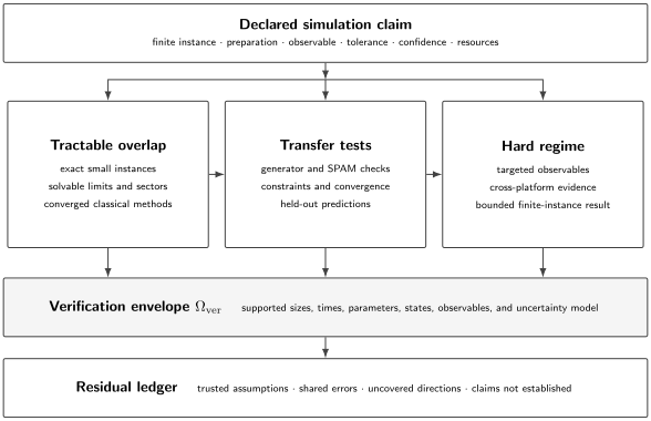
Trust is transferred from tractable overlap to the hard regime through tests of the implemented generator, structural identities, convergence, and held-out predictions. The final claim is restricted to the verified observables and operating envelope; assumptions and uncovered directions remain visible.

The envelope is not the convex hull of every tested point. If a path crosses a phase transition, resonance, heating threshold, loss of controllability, or change in classical approximation quality, interpolation may fail. Every extension from a checked regime to an unchecked one needs a transport argument.

Verification Is a Dependency Graph

The final result depends on several propositions:

$$\begin{gathered} \text{target definition} \longrightarrow \text{encoding or model reduction} \longrightarrow \text{implemented dynamics} \\ \longrightarrow \text{state preparation} \longrightarrow \text{measurement record} \longrightarrow \text{estimator and claim}. \end{gathered}$$

Each edge can fail while downstream plots remain plausible. A verification dossier should therefore record:

$$\mathcal V = \left( \mathcal T, \mathcal E, \mathcal A, \mathcal B, \Omega_{\mathrm{ver}} \right),$$

where $\mathcal T$ is the set of tests, $\mathcal E$ their outcomes and uncertainties, $\mathcal A$ the trusted assumptions, and $\mathcal B$ the remaining discrepancy or error budget.

An attractive test is not necessarily a useful test. For every test $T_k$, write down:

1. which dependency edge it probes;
2. which error mechanisms can make it fail;
3. which error mechanisms can pass unnoticed;
4. whether its data were used for calibration or model selection;
5. the operating region over which its conclusion applies.

Trusted Boundary and Assumption Ledger

No verification protocol is assumption free. Even a formally device- independent protocol trusts randomness, isolation, or communication structure. Simulation experiments commonly trust some combination of:

• the identification of physical degrees of freedom;
• locality or sparsity of the generator ansatz;
• independence or exchangeability of repeated preparations;
• calibrated measurement operators;
• a Hilbert-space truncation and leakage model;
• a Markovian, stationary, or weak-noise description;
• classical numerical reference calculations and software;
• absence of adversarial behavior;
• a complexity-theoretic conjecture for an advantage claim.

Assumptions should be classified as tested, externally calibrated, theoretically justified, or unverified. The distinction matters. A fit that assumes nearest-neighbor interactions cannot use a small residual as evidence that longer-range terms are absent unless those alternatives were tested.

Method Selector

Method	Best use	What it can establish	Main blind spot
exact small-instance comparison	finite states or dynamics	end-to-end agreement in overlap regime	size- or time-dependent errors
solvable limits	parameter endpoints and special sectors	correct conventions and limiting behavior	off-limit interactions
short-time expansion	local dynamics and generator moments	early-time derivatives	accumulated long-time error
conserved quantities and constraints	symmetries, gauge laws, continuity	necessary structural consistency	symmetry-preserving errors
convergence and sensitivity	digital step, cutoff, ramp, size, analysis	stability under a chosen refinement	common bias across refinements
Hamiltonian or channel learning	structured implemented dynamics	parameters and held-out predictions	ansatz misspecification
targeted fidelity or witness	a state property	property-specific certificate	other state features
tomography or shadows	state or selected observables	reconstruction or many estimates	scaling and measurement trust
benchmark-model family	complete workflow	coverage of chosen failure modes	unrepresented target regimes
cross-platform comparison	independent implementations	consistency and discrepancy localization	shared target or analysis error
blind held-out prediction	transfer beyond fitting data	predictive model adequacy	limited holdout coverage

A strong verification package uses methods with different blind spots. Ten tests of the same conserved quantity are not ten independent lines of evidence.

Exact Classical Comparison

Direct comparison remains the cleanest check where it is feasible. For a reference prediction $\mu_{\mathrm{ref}}$ and experimental estimate $\widehat\mu$, define a discrepancy

$$r = \widehat\mu-\mu_{\mathrm{ref}}.$$

The uncertainty of $r$ includes both sides,

$$u_r^2 = u_{\mathrm{exp}}^2 + u_{\mathrm{ref}}^2 - 2\operatorname{Cov} \left( \widehat\mu, \mu_{\mathrm{ref}} \right).$$

Classical reference uncertainty may include finite precision, truncation, solver convergence, Monte Carlo sampling, finite bond dimension, or model parameter uncertainty. Calling a numerical answer exact does not make the implementation or input data exact.

Use the strongest applicable method

Exact diagonalization is only one reference. Depending on the instance, useful methods include:

• free-particle and stabilizer reductions;
• tensor networks at limited entanglement or time;
• sign-problem-free Monte Carlo;
• Krylov and sparse-matrix propagation;
• perturbative, semiclassical, or mean-field limits with controlled errors;
• symmetry decomposition and reduced sectors;
• interval, variational, or rigorous upper and lower bounds.

The relevant comparison is with the best method for the same input, observable, and tolerance. A classical method that cannot reconstruct the full state may still compute the local observable being claimed.

Compare distributions, not only means

Agreement of one expectation value can hide state error. When feasible, compare a vector of observables, marginal distributions, time correlations, or raw bitstring statistics. A quadratic discrepancy with covariance $\Sigma$ is

$$\chi^2 = \mathbf r^{\mathsf T} \Sigma^{-1} \mathbf r.$$

Its interpretation requires a justified covariance model and degrees of freedom. If parameters were fitted to the same data, the naive reference distribution for $\chi^2$ is generally wrong.

Small size does not automatically transfer

Suppose sizes $L\leq L_0$ agree. Larger systems may activate crosstalk, inhomogeneity, long-range tails, heating, calibration congestion, or error growth with volume. Transfer to $L>L_0$ requires tests that are sensitive to those mechanisms, not merely more precise agreement below $L_0$.

Limiting Cases and Tractable Deformations

A target family $H(\lambda)$ often contains points with known solutions. Good limits isolate different terms:

• zero interaction;
• zero hopping or decoupled sites;
• one-particle and two-particle sectors;
• high-field, weak-coupling, or atomic limits;
• integrable lines;
• infinite-temperature or short-time limits;
• vanishing drive or dissipation;
• small graph motifs with exact spectra.

The limit should be reached through the same control and measurement pipeline as the hard experiment. Replacing the apparatus with a separate easy implementation may test analysis code without testing the relevant controls.

Metamorphic relations

Some tests need no full reference answer. A transformation of the input may imply a transformation of the output. Examples include:

• permuting equivalent sites;
• reversing a field and applying a known basis transformation;
• changing units or rotating frames;
• reversing time for a reversible ideal model;
• duplicating disconnected components;
• applying a gauge transformation while preserving gauge-invariant outputs.

These metamorphic tests can expose sign, indexing, frame, and compilation errors. They verify the relation, not either output absolutely.

Short-Time Expansions

For a closed target and observable $O$,

$$\langle O(t)\rangle = \langle O\rangle_0 + \frac{it}{\hbar} \langle[H,O]\rangle_0 - \frac{t^2}{2\hbar^2} \langle[H,[H,O]]\rangle_0 + O(t^3).$$

The first derivatives depend only on local commutator structure for local Hamiltonians. They can be calculated even when long-time dynamics is hard. Measuring several initial states and observables turns these derivatives into tests of generator terms and sign conventions.

Short-time agreement has a strict scope. Coherent errors may accumulate, dissipation may dominate later, and two generators with matching first few moments can diverge at longer times. The expansion is a generator diagnostic, not a long-time certificate.

Conserved Quantities, Constraints, and Sum Rules

If $[H,Q]=0$, then ideal closed evolution preserves

$$\langle Q(t)\rangle = \langle Q(0)\rangle.$$

Violations can reveal leakage, symmetry-breaking controls, loss, drift, or incorrect reconstruction. The same logic applies to:

• particle number, parity, energy, and total spin;
• Gauss-law constraints in gauge simulations;
• local continuity equations;
• normalization and positivity;
• spectral and response-function sum rules;
• causal or locality bounds;
• thermodynamic identities.

For local density $n_i$ and current $j_{i\to j}$, a continuity residual is

$$R_i(t) = \frac{d}{dt}\langle n_i(t)\rangle + \sum_j \langle j_{i\to j}(t)\rangle.$$

The ideal residual vanishes after boundary sources and sinks are included. Testing local residuals is often more diagnostic than testing only total number, because spatially correlated errors can conserve the total.

Necessary is not sufficient

A simulator evolving under the wrong Hamiltonian can preserve the same symmetry. Depolarization within a fixed sector can pass a charge check. A readout correction can enforce normalization while biasing correlations. Structural identities are powerful falsifiers, but passing them rarely identifies the full state or generator.

Convergence and Sensitivity Tests

Verification should vary controls that change a known approximation while holding the target fixed.

Digital refinements

Vary product-formula step size, compilation, synthesis precision, logical cutoff, ancilla precision, or mitigation strength. A target estimator may have an expansion

$$\widehat\mu(\delta) = \mu_0 + c\delta^p + O(\delta^{p+1}) + b_{\mathrm{hw}}(\delta).$$

Hardware error $b_{\mathrm{hw}}$ can grow as $\delta$ decreases because the circuit becomes deeper. Monotonic convergence is therefore not guaranteed; the model must include both trends.

Analog refinements

Vary ramp speed, drive frequency, interaction cutoff, temperature, disorder realization, lattice spacing, boundary, and evolution window. Since analog hardware does not have a universal step size, refinement must be tied to the specific effective-model approximation.

Numerical and analysis refinements

Vary Fock cutoff, bond dimension, time step, fit window, regularization, response model, and bootstrap unit. Stability under analysis choices is evidence against one class of bias, but several methods can share the same incorrect input model.

Negative controls

A verifier should fail when a known fault is injected. Deliberately perturb a coupling, violate a symmetry, add leakage, scramble a phase, or distort a readout model. If the chosen metrics do not respond at the scientifically relevant fault scale, they cannot support the main claim.

Learning the Implemented Generator

For a structured Hamiltonian ansatz

$$H(\boldsymbol\theta) = \sum_{a=1}^{m}\theta_a P_a,$$

short-time slopes obey

$$\left. \frac{d}{dt} \langle O_b(t)\rangle \right|_{t=0} = \frac{i}{\hbar} \sum_a \theta_a \langle[P_a,O_b]\rangle_0.$$

For several states and observables this becomes a linear inverse problem

$$\mathbf y = A\boldsymbol\theta + \boldsymbol\eta.$$

The singular values of $A$ determine which parameter combinations are identifiable. A small singular value amplifies statistical and calibration error. More data do not fix an unidentifiable design if the new rows of $A$ carry the same information.

Model testing, not only parameter fitting

Generator learning is conditional on the basis $\{P_a\}$. A mature workflow compares nested or alternative ansatzes, inspects structured residuals, and tests predictions on states, times, and observables not used in fitting. It also propagates the posterior or confidence region for $\boldsymbol\theta$ to the target observable.

Open-system inference replaces $H$ by a channel or Liouvillian ansatz. The physicality, memory, and time dependence of that ansatz then become additional tests. A fitted Markovian generator cannot rule out non-Markovian dynamics outside the fitted time resolution.

Targeted State and Property Verification

Full tomography of $n$ generic qubits requires exponentially many parameters. Simulation verification should therefore target the property needed for the claim whenever possible.

Direct fidelity estimation

If an efficiently described pure target $|\psi\rangle$ is available, its fidelity with an experimental state $\rho$ is

$$F = \langle\psi|\rho|\psi\rangle.$$

Importance-sampled Pauli measurements can estimate this quantity without full tomography for suitable targets. The protocol certifies closeness to the specified state, not correctness of an unknown state in a classically hard regime where the target description itself is unavailable.

Witnesses and local marginals

Entanglement witnesses, stabilizers, parent-Hamiltonian energies, and local reduced states can certify selected structure. Their power depends on a gap, uniqueness, locality, or another model property. A witness that detects entanglement does not identify the phase or validate the dynamics that prepared it.

Structure-assisted tomography

Matrix-product-state or compressed reconstruction can be efficient for states with limited entanglement or low rank. The structural assumption must itself be checked with a certificate or residual. If the hard regime produces volume-law entanglement, a low-bond-dimension reconstruction may fit local data while missing global structure.

Classical shadows

Randomized measurements can estimate many predeclared or postselected properties from a shared data set. A schematic sample bound is

$$N \gtrsim \frac{ \max_j \lVert O_j\rVert_{\mathrm{sh}}^2 }{\epsilon^2} \log\left(\frac{M}{\alpha}\right),$$

where the shadow norm depends on the measurement ensemble and observables. The logarithmic dependence on the number $M$ of observables does not remove the potentially large shadow norm, control noise, leakage, or classical post-processing cost.

Energy and Variance Certificates

Ground-state simulation sometimes permits a certificate without knowing the full state. Let $H$ have ground-space projector $P_0$, ground energy $E_0$, and a gap $\Delta>0$ to every state outside that space. Then

$$H \succeq E_0P_0 + (E_0+\Delta)(I-P_0).$$

For any state $\rho$ with energy $E=\operatorname{Tr}(H\rho)$,

$$\operatorname{Tr}(P_0\rho) \geq 1- \frac{E-E_0}{\Delta}.$$

If local terms of $H$ are measurable and $E_0$ and $\Delta$ are trusted, the energy gives a ground-space fidelity bound. The guarantee weakens when the gap is small or uncertain. It certifies the ground space, not a unique state when the ground space is degenerate.

The energy variance

$$\operatorname{Var}_\rho(H) = \langle H^2\rangle_\rho - \langle H\rangle_\rho^2$$

vanishes for an exact eigenstate. Small variance can bound spectral spread, but it does not identify which eigenstate was prepared. A high-energy eigenstate also has zero variance. Energy location, spectral isolation, and generator calibration are indispensable.

Cross-Platform Verification

Two devices can implement the same target with different microscopic errors. Randomized local measurements can estimate

$$\operatorname{Tr}(\rho_A\rho_B), \qquad \operatorname{Tr}(\rho_A^2), \qquad \operatorname{Tr}(\rho_B^2),$$

and hence the Hilbert–Schmidt distance

$$\lVert\rho_A-\rho_B\rVert_2^2 = \operatorname{Tr}(\rho_A^2) + \operatorname{Tr}(\rho_B^2) - 2\operatorname{Tr}(\rho_A\rho_B).$$

This can compare states without reconstructing either one fully. In large Hilbert spaces, small Hilbert–Schmidt distance does not automatically imply a strong trace-distance guarantee; the chosen metric must match the claim.

Independence is a scientific design choice

Cross-platform agreement is strongest when the devices differ in encoding, control, measurement, and dominant noise. It is weaker if both use the same calibration code, target-map convention, classical fit, or post-processing library. Shared errors create covariance and can make apparent agreement more likely.

Disagreement is useful. By comparing easy limits, local sectors, and response to controlled perturbations, one can often identify whether the discrepancy comes from target conventions, state preparation, dynamics, measurement, or analysis.

Benchmark Models and Coverage

A benchmark model family is a set of falsifiable contracts chosen to exercise distinct parts of the simulation pipeline. A useful family includes:

1. zero- and one-body limits for signs and local controls;
2. small interacting instances for end-to-end exact comparison;
3. symmetry sectors and constrained models for leakage detection;
4. integrable or free lines for larger-size checks;
5. nonintegrable finite instances for interaction and sampling stress;
6. open-system cases for loss, reset, and steady-state handling;
7. hidden instances reserved for prediction rather than fitting.

Coverage should be recorded as a matrix of failure mechanisms versus tests. Passing a benchmark suite establishes performance on its contracts. It does not prove correctness for every Hamiltonian in the same broad model class.

The Many-Body Benchmark Problems page supplies fixed finite-model contracts. Validation Tests owns the sitewide executable-test taxonomy.

Held-Out and Blind Prediction

Calibration and validation data serve different statistical roles. If a model is fitted on all measured times and observables, agreement with those records is in-sample description, not independent prediction.

A held-out design may reserve:

• later times;
• unseen initial states;
• different observables;
• hidden coupling patterns;
• new system sizes;
• disorder realizations sampled after model freezing;
• a second laboratory or analysis team.

The model, preprocessing, exclusion rules, and acceptance thresholds should be frozen before the held-out outcomes are revealed. Repeatedly inspecting a holdout and updating the model turns it into training data.

Interpolation is easier than extrapolation

A randomly withheld point inside a densely sampled calibration region mainly tests interpolation. To test transfer toward the hard regime, choose holdouts that stress the intended direction: larger size, longer time, stronger interaction, different geometry, or a more nonlocal observable. The step must remain small enough that failure is diagnostically useful.

Propagating Error to the Claimed Observable

Verification evidence becomes useful only after it bounds the output of interest.

State distance

For trace distance

$$D(\rho,\sigma) = \frac12 \lVert\rho-\sigma\rVert_1,$$

any bounded observable satisfies

$$\left| \operatorname{Tr}[O(\rho-\sigma)] \right| \leq 2\lVert O\rVert_\infty D(\rho,\sigma).$$

A global state-distance bound is strong but often expensive. A direct bound for one local observable can be much cheaper and more relevant.

Hamiltonian discrepancy

Let $H'=H+\Delta H$, with the same initial state. Duhamel’s formula gives

$$e^{-iH't/\hbar} - e^{-iHt/\hbar} = -\frac{i}{\hbar} \int_0^t e^{-iH'(t-s)/\hbar} \Delta H e^{-iHs/\hbar} \,ds.$$

Therefore

$$\left\lVert e^{-iH't/\hbar} - e^{-iHt/\hbar} \right\rVert \leq \frac{t}{\hbar} \lVert\Delta H\rVert.$$

A conservative observable bound is

$$|\Delta\langle O\rangle| \leq 2\lVert O\rVert_\infty \min\left\lbrace 1, \frac{t}{\hbar}\lVert\Delta H\rVert \right\rbrace.$$

This global operator-norm bound often scales poorly with system size. Locality, Lieb–Robinson bounds, perturbation theory, or observable-specific response can give sharper estimates. A loose rigorous bound and a small empirical residual answer different questions and should not be merged without explanation.

Open-system discrepancy

For two contractive Markovian semigroups with generators $\mathcal L$ and $\mathcal L+\Delta\mathcal L$, a corresponding induced trace-norm estimate is

$$\left\lVert e^{t(\mathcal L+\Delta\mathcal L)} - e^{t\mathcal L} \right\rVert_{1\to1} \leq t\lVert\Delta\mathcal L\rVert_{1\to1},$$

under the stated contraction assumptions. Non-Markovian memory, initial system–environment correlations, and time-dependent generators need a different analysis.

Combine errors with their dependence structure

An additive ledger

$$\epsilon_{\mathrm{tot}} \leq \epsilon_{\mathrm{model}} + \epsilon_{\mathrm{impl}} + \epsilon_{\mathrm{prep}} + \epsilon_{\mathrm{meas}} + \epsilon_{\mathrm{stat}}$$

is safe when each term is a compatible worst-case bound. Standard uncertainties should not simply be added as if they were worst-case errors, and worst-case bounds should not be combined in quadrature as if independent Gaussian fluctuations. Correlation and shared calibration parameters matter.

Statistical Design

Define the independent unit

Thousands of shots acquired during one calibration interval may not be thousands of independent device realizations. Drift, common-mode noise, and batch effects make the run, day, chip, or disorder realization the relevant unit for some claims.

Separate exploration and confirmation

Choose primary observables, thresholds, exclusion rules, fit models, and holdouts before confirmatory analysis. Exploratory plots remain valuable, but their error bars do not account for all choices made after seeing the data.

Account for many checks

Testing many times, sites, observables, and analysis variants increases the chance of finding an apparent success or failure. Simultaneous confidence regions, hierarchical models, false-discovery controls, or predeclared families may be appropriate. Selecting the best-matching observable after the experiment is not the same as predicting it.

Passing tests do not multiply into a probability of correctness

If three tests pass with nominal $95\%$ coverage, one cannot conclude that the simulation is correct with probability $0.95^3$ or any other simple product. The tests are conditional on models, can be correlated, and may not cover all failure modes. Their combination is an evidence argument unless a formal joint certification theorem has been established.

Worked Example: Transverse-Field Ising Dynamics

Consider an open chain

$$H = -J\sum_{i=1}^{L-1}Z_iZ_{i+1} -h\sum_{i=1}^{L}X_i,$$

prepared in $|0\rangle^{\otimes L}$. Suppose the target outputs are

$$m_z(t) = \frac1L\sum_i\langle Z_i(t)\rangle$$

and connected correlations

$$C_{ij}(t) = \langle Z_i(t)Z_j(t)\rangle - \langle Z_i(t)\rangle \langle Z_j(t)\rangle.$$

The desired frontier regime has larger $L$ and later $t$ than exact diagonalization permits.

Layer 1: conventions and limits

At $h=0$, the initial state is an eigenstate and

$$m_z(t)=1, \qquad C_{ij}(t)=0.$$

At $J=0$, independent spins give

$$m_z(t) = \cos\left(\frac{2ht}{\hbar}\right),$$

and connected correlations remain zero. These limits test field calibration, sign and factor conventions, time conversion, local rotations, and readout.

Layer 2: short-time moments

For the chosen initial state,

$$\left. \frac{d}{dt}m_z(t) \right|_{t=0} = 0,$$

and

$$\left. \frac{d^2}{dt^2}m_z(t) \right|_{t=0} = -\frac{4h^2}{\hbar^2}.$$

The interaction does not enter this particular second derivative because the initial expectation values of the relevant $X_iZ_j$ terms vanish. Interaction calibration therefore needs other states, higher moments, or correlation growth; fitting only $m_z(t)$ near zero is not sufficient to identify $J$.

Layer 3: structural checks

The global spin-flip operator

$$P = \prod_{i=1}^{L}X_i$$

commutes with $H$. Prepare parity eigenstates to test sector preservation. Energy is conserved under the ideal time-independent closed evolution. Local correlation fronts can also be compared with locality bounds. Passing these checks does not exclude a wrong parity-preserving nearest-neighbor coupling.

Layer 4: exact overlap

For small $L$, compare complete bitstring distributions, $m_z(t)$, $C_{ij}(t)$, and selected basis-rotated observables with exact propagation. Freeze readout correction and Hamiltonian parameters before evaluating held- out times and initial states.

Layer 5: tractable deformation

The one-dimensional model is integrable after a Jordan–Wigner transformation, which permits larger classical checks for this Hamiltonian. To verify a nonintegrable extension, introduce a longitudinal field or other perturbation gradually and compare with tensor-network calculations over their converged time window. Report where bond-dimension or truncation convergence fails.

Layer 6: hard-regime transfer

At larger size and later time, retain local generator checks, symmetry tests, injected-fault sensitivity, cross-platform observables where available, and multiple classical approximations with overlapping windows. The final claim should concern the measured observables and finite instances. It should not say that the full many-body wavefunction has been verified.

A Verification Package for a Hard Regime

A practical package can be organized as follows.

Target and estimand

• finite instance, boundaries, model parameters, and preparation;
• primary observables and time or frequency windows;
• acceptance tolerance and uncertainty semantics.

Implementation evidence

• independently calibrated controls and measurements;
• inferred generator with uncertainty and alternative ansatz tests;
• leakage, loss, drift, and context dependence under the actual protocol.

Overlap evidence

• exact small sizes and solvable limits;
• converged classical approximations over stated windows;
• short-time moments and few-excitation sectors.

Structural evidence

• conservation laws, constraints, continuity, and sum rules;
• known invariances and metamorphic relations;
• negative controls and injected faults.

Transfer evidence

• size, time, parameter, and refinement trends;
• held-out predictions toward the hard regime;
• stability under alternate analysis and reference methods.

Independent evidence

• cross-platform or cross-encoding comparison;
• independent data analysis or laboratory reproduction;
• archived raw records, metadata, and code sufficient to audit the claim.

Residual statement

• uncovered observables and parameter directions;
• assumptions not directly tested;
• worst-case and statistical error components;
• claims explicitly not supported by the evidence.

Common Mistakes

Treating agreement as proof

Two wrong implementations can agree. Agreement becomes informative only after shared assumptions and correlated errors are examined.

Treating a necessary condition as sufficient

Conserving parity, particle number, or energy rules out some faults. It does not identify the state or Hamiltonian uniquely.

Verifying the easy task and claiming the hard one

Agreement at small size, short time, weak coupling, or for local observables does not automatically verify larger size, longer time, strong coupling, or a global property.

Fitting and testing on the same data

A flexible Hamiltonian, noise model, or mitigation rule can absorb the records used to construct it. Held-out prediction tests transfer.

Using tomography as a ritual

Full reconstruction may be infeasible or unnecessary. Conversely, a structure-assisted reconstruction is not assumption free. Measure what the claim needs and validate the structural prior.

Ignoring reference uncertainty

Tensor-network, Monte Carlo, perturbative, and exact-diagonalization software have finite precision, truncation, sampling, and implementation error.

Choosing the verification metric after seeing results

Selecting the observable, time window, normalization, or distance that looks best introduces selection bias. Exploratory and confirmatory claims should be distinguished.

Relabeling uncontrolled noise as target physics

Observed dissipation supports an open-system simulation only when the target channel is specified and unwanted channels are bounded.

Calling classical hardness verification

The inability of one classical method to compute an answer does not make the quantum answer correct. Correctness and classical hardness are separate propositions.

Reporting a fidelity without its trust boundary

A fidelity estimate depends on a target, measurement model, estimator, state family, and uncertainty. It is not a platform-independent seal of correctness.

What Can Be Claimed

The evidence level should determine the grammar of the result.

Evidence	Defensible wording
component tests only	“the controls and measurements meet the stated specifications”
exact overlap only	“the workflow reproduces these finite reference instances”
generator plus held-out agreement	“the calibrated model predicts these states, times, and observables”
property certificate	“the prepared state has at least the stated overlap or property under the certificate assumptions”
cross-platform agreement	“independent implementations agree for these comparison observables”
layered hard-regime package	“the reported finite-instance observable is supported by the stated verification envelope”

Claims about a thermodynamic phase, continuum limit, real material, or quantum advantage need additional scaling, model-validation, or complexity evidence.

Research Status

Small-system classical comparison, symmetry checks, local calibration, tomography, targeted witnesses, and benchmark models are established tools. Randomized measurements, structure-assisted reconstruction, cross-platform overlaps, local-Hamiltonian learning, and energy-based certificates have rigorous formulations and experimental demonstrations under stated assumptions.

Scalable end-to-end verification of generic, long-time, strongly interacting quantum dynamics remains an active problem. There is no general efficient classical protocol that certifies every useful output of an arbitrary quantum simulator; such a protocol would undermine the computational motivation for many simulations. Progress instead comes from task structure, restricted observables, interaction with a prover, multiple devices, trusted local measurements, or model-specific certificates.

Machine-learned state and generator models are increasingly useful for prediction and anomaly detection. Their uncertainty, distribution shift, training-data dependence, and physical constraints must be validated like any other model. A highly accurate predictor on sampled settings is not by itself a certificate outside that distribution.

Reporting Checklist

1. What exact finite target, observable, and tolerance are claimed?
2. Which verification, validation, certification, and benchmarking questions are being answered?
3. What is the verification envelope in size, time, parameter, state, and observable space?
4. Which assumptions are tested, calibrated, theoretical, or unverified?
5. What does each test falsify, and what can pass unnoticed?
6. Which data selected or fitted the model, and which data were held out?
7. What uncertainty belongs to classical references and post-processing?
8. How do results change under refinements, perturbations, and injected faults?
9. How are generator, state, measurement, and statistical errors propagated to the primary observable?
10. Which broader claims are not supported by the present evidence?

References

1. P. Hauke, F. M. Cucchietti, L. Tagliacozzo, I. Deutsch, and M. Lewenstein, “Can one trust quantum simulators?” Reports on Progress in Physics 75, 082401 (2012), doi:10.1088/0034-4885/75/8/082401.
2. J. Eisert et al., “Quantum certification and benchmarking,” Nature Reviews Physics 2, 382–390 (2020), doi:10.1038/s42254-020-0186-4.
3. J. Carrasco, A. Elben, C. Kokail, B. Kraus, and P. Zoller, “Theoretical and experimental perspectives of quantum verification,” PRX Quantum 2, 010102 (2021), doi:10.1103/PRXQuantum.2.010102.
4. M. Kliesch and I. Roth, “Theory of quantum system certification,” PRX Quantum 2, 010201 (2021), doi:10.1103/PRXQuantum.2.010201.
5. D. Hangleiter, M. Kliesch, M. Schwarz, and J. Eisert, “Direct certification of a class of quantum simulations,” Quantum Science and Technology 2, 015004 (2017), doi:10.1088/2058-9565/2/1/015004.
6. J. Bermejo-Vega, D. Hangleiter, M. Schwarz, R. Raussendorf, and J. Eisert, “Architectures for quantum simulation showing a quantum speedup,” Physical Review X 8, 021010 (2018), doi:10.1103/PhysRevX.8.021010.
7. S. T. Flammia and Y.-K. Liu, “Direct fidelity estimation from few Pauli measurements,” Physical Review Letters 106, 230501 (2011), doi:10.1103/PhysRevLett.106.230501.
8. M. Cramer et al., “Efficient quantum state tomography,” Nature Communications 1, 149 (2010), doi:10.1038/ncomms1147.
9. B. P. Lanyon et al., “Efficient tomography of a quantum many-body system,” Nature Physics 13, 1158–1162 (2017), doi:10.1038/nphys4244.
10. H.-Y. Huang, R. Kueng, and J. Preskill, “Predicting many properties of a quantum system from very few measurements,” Nature Physics 16, 1050–1057 (2020), doi:10.1038/s41567-020-0932-7.
11. A. Elben et al., “The randomized measurement toolbox,” Nature Reviews Physics 5, 9–24 (2023), doi:10.1038/s42254-022-00535-2.
12. A. Elben et al., “Cross-platform verification of intermediate scale quantum devices,” Physical Review Letters 124, 010504 (2020), doi:10.1103/PhysRevLett.124.010504.
13. E. Bairey, I. Arad, and N. H. Lindner, “Learning a local Hamiltonian from local measurements,” Physical Review Letters 122, 020504 (2019), doi:10.1103/PhysRevLett.122.020504.
14. X.-L. Qi and D. Ranard, “Determining a local Hamiltonian from a single eigenstate,” Quantum 3, 159 (2019), doi:10.22331/q-2019-07-08-159.
15. C. Kokail et al., “Self-verifying variational quantum simulation of lattice models,” Nature 569, 355–360 (2019), doi:10.1038/s41586-019-1177-4.

Exercises

1. Necessary versus sufficient tests

A gauge-theory simulator preserves Gauss’s law within measurement uncertainty for every reported time. Which claim is supported? Give two substantial errors that can pass this test.

Solution

The data support the bounded claim that the measured states remain in, or close to, the tested gauge-constraint sector under the stated measurement model. This is a necessary structural check. It does not verify the full Hamiltonian or state. An incorrect gauge-invariant coupling can preserve Gauss’s law, as can dephasing or mixing entirely within the physical sector. A readout model that projects records onto the physical sector could also produce apparent preservation. Additional generator, observable, and held-out checks are required.

2. Convert state distance to observable error

Two states satisfy $D(\rho,\sigma)\leq0.03$. Bound the discrepancy in the expectation of a Pauli string $P$. What bound follows for $O=(1/L)\sum_i Z_i$?

Solution

Every Pauli string has $\lVert P\rVert_\infty=1$, so

$$\left| \operatorname{Tr}[P(\rho-\sigma)] \right| \leq 2(1)(0.03) = 0.06.$$

The averaged magnetization also has operator norm at most one because the $Z_i$ commute and its eigenvalues lie in $[-1,1]$. Therefore the same global trace-distance information gives

$$|\Delta\langle O\rangle| \leq 0.06.$$

One should not add $L$ separate bounds; doing so would discard the norm of the averaged observable.

3. Propagate a Hamiltonian discrepancy

The calibrated Hamiltonian obeys $\lVert H_{\mathrm{dev}}-H_{\mathrm{tar}}\rVert\leq0.01\hbar/\tau$. Use the global bound on this page to bound the difference of a norm-one observable at $t=5\tau$. Why may this result be pessimistic?

Solution

The unitary difference is bounded by

$$\frac{t}{\hbar} \lVert\Delta H\rVert \leq 5\tau\frac{0.01\hbar/\tau}{\hbar} = 0.05.$$

Thus

$$|\Delta\langle O\rangle| \leq 2(1)(0.05) = 0.10.$$

The bound uses the global operator norm and allows the worst possible initial state and observable alignment. A local observable may be insensitive to distant terms over this time, errors may cancel, and a response calculation or locality bound may be much sharper. Those improvements require additional structure rather than simply replacing the rigorous number by an empirical one.

4. Ground-space energy certificate

A target Hamiltonian has known ground energy $E_0=-12.0$ and gap $\Delta=0.8$. A prepared state has energy $E=-11.76\pm0.04$. Give the nominal ground-space fidelity lower bound and a conservative bound using the upper end of the one-standard-uncertainty interval. State two assumptions.

Solution

Nominally,

$$\operatorname{Tr}(P_0\rho) \geq 1- \frac{-11.76+12.0}{0.8} = 0.70.$$

Using $E=-11.72$ gives

$$\operatorname{Tr}(P_0\rho) \geq 1- \frac{0.28}{0.8} = 0.65.$$

This latter number is not automatically a particular confidence bound unless the meaning of $0.04$ is specified. The argument assumes that the implemented and measured Hamiltonian is the target $H$ within accounted uncertainty and that $E_0$ and the spectral gap are valid for the finite sector and boundary conditions. If the ground space is degenerate, the certificate applies to the space, not a selected ground state.

5. Derive the Ising short-time curvature

For the worked Ising Hamiltonian and initial state $|0\rangle^{\otimes L}$, derive

$$\left. \frac{d^2}{dt^2} \langle Z_i(t)\rangle \right|_{t=0} = -\frac{4h^2}{\hbar^2}.$$

Why does this test not identify $J$?

Solution

The Heisenberg equation gives

$$\frac{dZ_i}{dt} = \frac{i}{\hbar}[H,Z_i] = -\frac{2h}{\hbar}Y_i.$$

Also,

$$\frac{dY_i}{dt} = \frac{2h}{\hbar}Z_i - \frac{2J}{\hbar} \sum_{j:\langle i,j\rangle} X_iZ_j.$$

Therefore

$$\frac{d^2Z_i}{dt^2} = -\frac{4h^2}{\hbar^2}Z_i + \frac{4hJ}{\hbar^2} \sum_{j:\langle i,j\rangle} X_iZ_j.$$

In the initial state, $\langle Z_i\rangle=1$ and $\langle X_iZ_j\rangle=0$, giving the stated curvature. Since the $J$-dependent expectation vanishes, this one state-observable pair has no second-order sensitivity to $J$. Other preparations, correlation functions, or higher derivatives are needed.

6. Audit a cross-platform agreement

Two platforms report the same correlator within $1\%$. Both use the same target-to-observable conversion code and the same fitted finite-temperature model. Give a verification conclusion and an improved design.

Solution

The result establishes consistency of the two complete pipelines for that correlator, conditional on the shared conversion and temperature model. It does not independently test those shared layers. An improved design would exchange more nearly raw observables, have separate teams implement the target-map and estimator, compare additional quantities with different model dependence, and use hidden instances or held-out parameters. A third reference method or an analytically controlled limit can test the shared convention.

7. Design a holdout toward the hard regime

A model is calibrated for sizes $L=6,8,10$ and times $tJ/\hbar\leq2$. The scientific result concerns $L=30$ at $tJ/\hbar=8$. Propose a staged holdout design more informative than randomly hiding $10\%$ of the calibration points.

Solution

Freeze the generator and analysis after the original calibration. First hold out new initial states and observables at $L=10$ to test model completeness. Then test unseen sizes such as $L=12,14$ over the classically converged time window. Separately extend time at fixed moderate size until the best classical method loses convergence, using overlapping methods and refinement tests near that boundary. Finally reserve selected combinations of larger size and later time, together with structural checks and injected faults, before evaluating the $L=30$ data. This staircase tests the two extrapolation directions and can localize failure; a random in-domain split mainly tests interpolation.

8. Write a bounded frontier claim

An experiment passes small-size exact comparisons, number conservation, step-size convergence, and held-out local correlators, then measures a new local correlator at a classically inaccessible size. Write a defensible claim and name one unsupported stronger claim.

Solution

A defensible statement is: “For the declared finite instance, preparation, time window, and local correlator, the reported estimate is supported by small-size end-to-end agreement, conserved-number tests, convergence over the tested step-size range, and held-out predictions of related local correlators, with the stated implementation and measurement error budget.” An unsupported stronger statement would be that the complete many-body state is correct, that all observables are verified, that the thermodynamic phase has been established, or that quantum advantage has been demonstrated. Each requires additional evidence.