Simulation of Lattice Gauge Theories

Short Definition

Quantum simulation of a lattice gauge theory is the controlled preparation, evolution, or interrogation of a spatially discretized gauge theory on a quantum device. Matter degrees of freedom usually live on sites, gauge fields on oriented links, and physical states satisfy a local Gauss constraint at every vertex. A complete simulation must preserve or quantify those constraints, control finite-dimensional link approximations, measure gauge-invariant observables, and state whether its claim concerns a finite lattice or a continuum quantum field theory.

Lattice gauge simulation is not obtained by taking an ordinary spin model and renaming a conserved quantity “gauge.” Gauge transformations are a redundancy, the physical Hilbert space is constrained locally, and link variables mediate parallel transport. These facts shape the register, gates, errors, observables, and validation strategy.

Canonical Scope

This page owns the Hamiltonian lattice-gauge-to-processor workflow:

• specifying matter, oriented links, gauge group, boundary flux, and Gauss-law sector;
• choosing explicit-link, constraint-eliminated, or gauge-invariant formulations;
• digitizing continuous gauge fields without confusing distinct finite models;
• compiling matter–gauge hopping, electric energy, and plaquette dynamics;
• preserving, protecting, or monitoring local gauge constraints;
• preparing vacua, charges, flux strings, and scattering or quench states;
• measuring charge, electric flux, Wilson lines and loops, string breaking, spectra, and real-time response;
• separating volume, lattice-spacing, gauge-field cutoff, algorithmic, hardware, and inference errors;
• identifying the additional renormalization and continuum evidence required for a field-theory claim.

From Phase Symmetry to Gauge Theory owns the conceptual distinction between global symmetry and gauge redundancy. Simulation of Lattice Models owns the generic graph-to-register workflow, term scheduling, state preparation, and finite-size validation shared by spin, fermion, and boson models. This page adds the specifically gauge-theoretic obligations.

A full field-theory treatment should remain the canonical home for continuum Yang–Mills theory, path integrals, renormalization, confinement, anomalies, fermion discretizations, and the phenomenology of quantum chromodynamics. Here those subjects appear only far enough to define a reproducible quantum simulation and an honest handoff to field theory.

Why Gauge Theories Are a Distinct Simulation Class

Three structures occur together.

1. Redundant description: gauge-related configurations represent the same physical state.
2. Local constraint: physical states satisfy one generator equation at each independent vertex.
3. Dynamical parallel transport: matter motion changes link flux so that the constraint remains satisfied.

Let $G_x^a$ generate a gauge transformation at vertex $x$, with $a$ a Lie algebra index for a non-Abelian group. In a charge sector $g_x^a$, physical states obey

$$G_x^a\lvert\psi_{\mathrm{phys}}\rangle = g_x^a\lvert\psi_{\mathrm{phys}}\rangle.$$

For a source-free sector, $g_x^a=0$. Gauge invariance of the ideal Hamiltonian means

$$[H,G_x^a]=0 \qquad \text{for every }x,a.$$

This is stronger than conservation of one global charge. A state can have the correct total charge while violating Gauss’s law locally at many vertices.

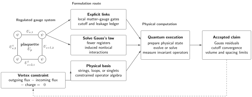
Matter lives on sites and gauge variables on oriented links. Gauss’s law ties the flux divergence at each vertex to local charge, while an oriented plaquette product supplies magnetic dynamics in two or more spatial dimensions. A quantum simulation may retain link registers, solve selected constraints and accept induced nonlocality, or work in a gauge-invariant string or loop basis. Each route has a different cutoff, compilation, and verification ledger.

Complete the Gauge-Theory Contract

A finite task can be summarized by

$$\mathcal G_L = \left( G, \Lambda_L, \mathcal H_{\mathrm m}, \mathcal H_{\mathrm g}, H_L, \{g_x^a\}, \rho_0, \mathcal Q, \boldsymbol\epsilon \right).$$

Here $G$ is the gauge group, $\Lambda_L$ is the finite oriented lattice, $\mathcal H_{\mathrm m}$ and $\mathcal H_{\mathrm g}$ are matter and gauge-link spaces, and $H_L$ is the regulated Hamiltonian. The selected Gauss sector is $\{g_x^a\}$, the input is $\rho_0$, and $\mathcal Q$ lists observables, times, or spectral quantities. The vector $\boldsymbol\epsilon$ records separate tolerances for finite volume, lattice spacing, link digitization, state preparation, evolution, hardware, sampling, and inference.

A reproducible contract also states:

• spatial dimension and lattice geometry;
• orientation convention for every link and plaquette;
• open, periodic, twisted, or fixed-flux boundary data;
• temporal gauge or other Hamiltonian gauge convention;
• matter discretization, flavor count, mass convention, and statistics;
• external charges and superselection sector;
• gauge-link basis and finite-dimensional approximation;
• bare couplings with lattice-spacing factors and units;
• whether the target is the regulated Hamiltonian or a continuum observable.

Hamiltonian Anatomy

Link variables and transformations

For a compact group, a link $\ell=(x,i)$ points from $x$ to $x+\hat i$ and carries a parallel transporter $U_{x,i}$. Under local transformations $\Omega_x\in G$,

$$U_{x,i} \longmapsto \Omega_x U_{x,i}\Omega_{x+\hat i}^{\dagger}.$$

Matter in the corresponding representation transforms as

$$\psi_x \longmapsto \Omega_x\psi_x.$$

Therefore the nearest-neighbor hopping operator

$$\psi_x^\dagger U_{x,i}\psi_{x+\hat i}$$

is gauge invariant. Omitting $U_{x,i}$ would compare internal orientations at different sites without parallel transport.

Electric generators

Non-Abelian links carry left and right electric generators. With one common convention,

$$[L^a,U]=T^aU, \qquad [R^a,U]=-UT^a,$$

where $T^a$ are representation generators. The two Casimirs agree on a link,

$$\sum_a L^aL^a = \sum_a R^aR^a.$$

Signs and whether incoming terms use $R^a$ or $-R^a$ vary across the literature. A simulation must state its convention and verify the local commutators rather than infer them from a diagram.

For compact $U(1)$, one may use an electric basis $\lvert\ell\rangle$, $\ell\in\mathbb Z$, with

$$E\lvert\ell\rangle = \ell\lvert\ell\rangle, \qquad U\lvert\ell\rangle = \lvert\ell+1\rangle,$$

so

$$[E,U]=U.$$

Plaquette holonomy

For an oriented elementary square in directions $i$ and $j$,

$$U_{p} = U_{x,i} U_{x+\hat i,j} U_{x+\hat j,i}^{\dagger} U_{x,j}^{\dagger}.$$

Its trace is gauge invariant because the vertex transformations cancel around the closed loop. In one spatial dimension there are no elementary spatial plaquettes, so a pure magnetic plaquette term is absent. This is one reason why 1+1-dimensional models are substantially simpler than higher-dimensional gauge theories.

Generic Kogut–Susskind structure

Suppressing convention-dependent lattice-spacing factors, a Hamiltonian with dynamical matter can be organized as

$$H = H_{\mathrm m} +H_{\mathrm{hop}} +H_E +H_B,$$

where

$$H_{\mathrm{hop}} = -w\sum_{x,i} \left( \psi_x^\dagger U_{x,i}\psi_{x+\hat i} +\mathrm{h.c.} \right),$$ $$H_E = \frac{g_E^2}{2} \sum_{\ell,a} (E_\ell^a)^2,$$

and a common magnetic term is

$$H_B = -\frac{1}{2g_B^2} \sum_p \left( \operatorname{Tr}U_p +\operatorname{Tr}U_p^\dagger \right).$$

The precise coefficients depend on spatial dimension, lattice spacing, group normalization, and whether constants have been subtracted. They must be copied from the declared regulated theory, not reconstructed from this schematic form.

Gauss’s Law as the Central Invariant

Abelian form

For oriented $U(1)$ links and site charge $Q_x$, define

$$G_x = \sum_{\ell\,\mathrm{out\ of}\,x}E_\ell -\sum_{\ell\,\mathrm{into}\,x}E_\ell -Q_x.$$

The source-free physical subspace satisfies

$$G_x\lvert\psi_{\mathrm{phys}}\rangle=0.$$

Summing over all sites cancels internal link fluxes. For periodic boundaries this imposes total charge zero unless the formulation includes an appropriate background. With open boundaries, total charge equals net outward boundary flux. Global consistency is therefore a boundary statement as well as a local one.

Non-Abelian form

For a non-Abelian group, the generator at $x$ combines outgoing left fields, incoming right fields, and matter color charge,

$$G_x^a = \sum_i \left( L_{x,i}^a +R_{x-\hat i,i}^a \right) -Q_x^a,$$

for the sign convention stated above. Physical states are local singlets or belong to sectors fixed by external color sources. The generators themselves do not all commute,

$$[G_x^a,G_y^b] = i\delta_{xy}f^{abc}G_x^c,$$

so simultaneous eigenvalue language must be used with care. The physical condition is annihilation by every generator in a source-free sector.

Constraint residuals

For an Abelian target sector $g_x$, a direct leakage diagnostic is

$$\epsilon_G = \frac1{N_v} \sum_x \left\langle (G_x-g_x)^2 \right\rangle.$$

It vanishes exactly only in the target sector. For non-Abelian groups, use a positive local Casimir residual, for example

$$\epsilon_G = \frac1{N_v} \sum_{x,a} \langle(G_x^a)^2\rangle$$

in the singlet sector. Report the normalization and cutoff dependence because the possible eigenvalues of $G_x^a$ depend on the link representation.

Low $\epsilon_G$ is necessary but not sufficient. Gauge-preserving coherent errors can alter physical dynamics while leaving every constraint exactly satisfied.

Three Formulation Routes

Retain explicit gauge links

The most direct formulation assigns registers to matter sites and gauge links. Local matter hopping changes both occupation and adjacent flux, while electric and plaquette terms act on links. Advantages include manifest spatial locality, direct access to flux observables, and a transparent approach to higher dimensions.

The costs are substantial:

• continuous groups require finite link registers;
• Gauss’s law reduces the physical space but does not automatically reduce the allocated register;
• a plaquette gate acts on at least four links before matter or ancillas;
• non-Abelian links carry representation and magnetic indices;
• hardware noise can leave the physical subspace.

Solve Gauss’s law

In one spatial dimension with open boundaries, Abelian Gauss’s law can be solved recursively. If $E_0$ is the left boundary flux and sites are ordered,

$$E_n = E_0+sum_{j=1}^{n}Q_j.$$

Substituting into the electric energy eliminates link variables,

$$H_E = \frac{g_E^2}{2} \sum_n \left( E_0+sum_{j\le n}Q_j \right)^2.$$

The register becomes smaller and every represented state can satisfy the solved constraints. The price is a long-range Coulomb interaction among charges. Boundary flux and total-charge compatibility must still be enforced, and the strategy does not generalize so simply to loops, higher dimensions, or non-Abelian groups.

This is an important locality tradeoff: eliminating redundant gauge registers can make the physical Hamiltonian less local on the remaining degrees of freedom.

Use a gauge-invariant basis

Loop, string, hadron, spin-network, prepotential, or related bases solve local singlet constraints at the level of basis states. They can reduce unphysical storage and make gauge-invariant ansätze natural. However, the resulting basis may have nontrivial global constraints, irregular state counting, complicated operators, or less transparent spatial locality.

There is no universally best basis. Compare formulations at fixed physical volume, link cutoff, target observables, and precision. A smaller Hilbert space can require a more expensive Hamiltonian oracle or more complicated state preparation.

Digitize Gauge Links Carefully

Hard electric-field cutoff

For compact $U(1)$, retain

$$-\Lambda\le\ell\le\Lambda, \qquad d_{\mathrm{link}}=2\Lambda+1.$$

A binary register needs

$$n_{\mathrm{link}} = \left\lceil \log_2(2\Lambda+1) \right\rceil$$

qubits, plus a convention for unused computational states. Projecting the shift operator onto this interval gives

$$U_\Lambda\lvert\ell\rangle = \begin{cases} \lvert\ell+1\rangle,&\ell<\Lambda,\\ 0,&\ell=\Lambda. \end{cases}$$

This finite operator is not unitary. The commutator and boundary algebra differ from the exact rotor. Convergence requires increasing $\Lambda$ and monitoring probability near both cutoff edges, not merely reporting link dimension.

Cyclic finite group

One can instead wrap the shift,

$$U_d\lvert d-1\rangle = \lvert0\rangle.$$

This preserves a finite Weyl algebra and describes a $\mathbb Z_d$ gauge theory. It is not the same finite model as a hard-truncated $U(1)$ rotor. A large-$d$ relation to $U(1)$ is a convergence claim that must be tested in the observable and coupling regime of interest.

Quantum-link and representation truncations

Quantum-link models replace infinite-dimensional link rotors by finite spin or rishon representations. For an Abelian example,

$$E=S^z, \qquad U\propto S^+.$$

Gauss’s law can remain exact while the link algebra changes at finite $S$. For non-Abelian compact groups, a Peter–Weyl link basis can be truncated to a finite set of irreducible representations,

$$\mathcal H_{\mathrm{link}} \simeq \bigoplus_{r\in\mathcal R_\Lambda} V_r\otimes V_r^*.$$

The retained representation set, multiplication rules after projection, and closure of compiled operators must be stated. “Three qubits per link” does not identify the gauge-field approximation.

Cutoff convergence is observable-dependent

Useful diagnostics include

$$p_{\mathrm{edge}} = \sum_{\ell\in\partial\mathcal E_\Lambda} \langle\ell\rvert\rho_{\mathrm{link}}\lvert\ell\rangle,$$

changes in the final observable under $\Lambda\to\Lambda+1$, and stability of low-energy spectra or transition amplitudes. Strong electric coupling can suppress high flux, while weak coupling and continuum approaches can require larger link spaces. A cutoff adequate for ground energy may fail for a violent real-time process that generates broad flux distributions.

Preserve the Gauge Constraint in Execution

Exact preservation by encoding

The strongest option is to represent only physical states. If an isometry $V:\mathcal H_{\mathrm{phys}}\to\mathcal H_{\mathrm{reg}}$ embeds the physical space, every logical operation should satisfy

$$U_{\mathrm{reg}}V = VU_{\mathrm{phys}}.$$

Gauge leakage is then excluded at the logical level. The tradeoff is that encoded operators can become nonlocal or expensive, and an invalid hardware operation can leave the code space unless the encoding detects it.

Exact preservation by primitive gates

With explicit links, construct every compiled generator $K_a$ so that

$$[K_a,G_x^b]=0 \qquad \text{for all }a,x,b.$$

Then each factor $e^{-iK_a\delta t}$ preserves the physical subspace at every intermediate time. A product formula assembled from these factors remains exactly gauge invariant even at finite step size,

$$[U_{\mathrm{PF}}(t),G_x^b]=0.$$

This requires compiling a gauge-invariant matter–link hop as one logical primitive or as a sequence whose full action and intermediate leakage are controlled. Splitting it into bare matter hopping and a separate link shift creates gauge-violating intermediate operators even when their product approaches the right Hamiltonian asymptotically.

Energy penalties

Add a positive penalty,

$$H_{\mathrm{pen}} = \lambda \sum_{x,a} (G_x^a-g_x^a)^2.$$

For sufficiently large $\lambda$, gauge-violating states are energetically separated. This can suppress weak perturbative transitions, but it is not free error correction. A finite penalty modifies off-shell dynamics, increases the Hamiltonian norm and digital simulation cost, and can create calibration or spectral-resolution demands. Resonant noise can still cross the penalty gap.

Penalty convergence must be demonstrated in the final observable while checking both leakage and in-sector distortion. Taking $\lambda$ as large as hardware allows is not automatically optimal.

Linear protection and constrained dynamics

A protection term of the form

$$H_{\mathrm{prot}} = V\sum_x c_x(G_x-g_x)$$

can energetically distinguish gauge sectors with fewer-body controls in some Abelian implementations. The coefficients $c_x$ must separate the relevant violations; uniform coefficients may protect only total charge. Quantum-Zeno, dissipative, and dynamical-decoupling strategies can also confine evolution to a target sector under specific time-scale assumptions.

Every protection scheme needs a residual effective Hamiltonian. If $H=H_0+H_{\mathrm{err}}+H_{\mathrm{prot}}$, state the leading in-sector terms generated by virtual excursions, not only the observed suppression of $\epsilon_G$.

Detection and postselection

If all $G_x$ or commuting stabilizer-like functions of them are measurable, one can reject records outside the target sector. With acceptance probability $p_{\mathrm{acc}}$, obtaining $N_{\mathrm{acc}}$ accepted shots costs on average

$$N_{\mathrm{raw}} = \frac{N_{\mathrm{acc}}}{p_{\mathrm{acc}}}.$$

Postselection does not detect errors that act entirely within the physical space. It can also bias time traces if acceptance depends strongly on the state or observable. Report raw and conditioned results, acceptance with uncertainty, and the prespecified acceptance rule.

Compile the Gauge Hamiltonian

Mass and electric energy

Mass, staggered-density, and Abelian electric-energy terms are diagonal in occupation and electric bases. Binary encodings implement them through phase polynomials or arithmetic; unary and qudit encodings can use level-dependent phases. The resource depends on coefficient precision and link dimension, not only the number of terms.

Matter–gauge hopping

A gauge-covariant hop has the schematic action

$$\lvert n_x,e,n_y\rangle \longleftrightarrow \lvert n_x-1,e+\delta e,n_y+1\rangle,$$

where $\delta e$ is fixed by orientation, matter charge, and representation. The update must be coherent and conditional on valid occupations and link boundaries. In a binary encoding it generally requires arithmetic or a multi-register select operation. In a native qudit implementation it can be a mixed-dimensional controlled rotation.

The hopping sign also contains fermionic parity information. In more than one dimension, the Jordan–Wigner or alternative fermion map can add strings even when the gauge link is geometrically adjacent. Gauge locality and fermionic encoding locality must be audited together.

Plaquette dynamics

The plaquette operator changes a closed loop of link flux. For $U(1)$,

$$U_p+U_p^\dagger$$

raises the oriented circulation around $p$ or lowers it. A digital implementation can use an ancilla to compute allowed shifts, apply a phase or rotation, and uncompute; direct qudit gates or analog ring exchange are other possibilities. Adjacent plaquettes share links, so plaquette scheduling is a hypergraph-coloring problem rather than ordinary edge coloring.

Product-formula groups

A useful split keeps each group gauge invariant,

$$H = H_{\mathrm{diag}} +H_{\mathrm{hop}}^{(1)} +\cdots +H_{\mathrm{hop}}^{(c_h)} +H_{\mathrm{plaq}}^{(1)} +\cdots.$$

Here direction, parity, or graph coloring creates internally parallel groups. The formula error is controlled by commutators among overlapping groups, while the exact Gauss symmetry survives finite step size if every group commutes with the generators. Trotter–Suzuki Methods develops the general error analysis.

Block encodings and fault-tolerant algorithms

Sparse-Hamiltonian, linear-combination, qubitization, and interaction-picture algorithms can improve asymptotic precision dependence. Their application cost is determined by the actual SELECT and PREPARE oracles for group-valued link updates, coefficients, plaquette products, and fermion signs. An oracle query is not one elementary gate.

The cutoff affects both the Hamiltonian norm and oracle arithmetic. A resource comparison must use the same physical volume, bare parameters, link digitization, target observable, and total error. Otherwise a favorable query count can describe a different regulated theory.

Prepare Physical States

Strong-coupling vacuum

When electric energy dominates, a simple vacuum often minimizes link flux and fills staggered matter sites according to the mass convention. It can be a product state satisfying Gauss’s law. This gives a valuable preparation starting point and a solvable validation limit.

The “vacuum” depends on regulator, boundary flux, mass sign, and background charge. A bare product vacuum is not the interacting continuum vacuum.

Charges and flux strings

An isolated charge is incompatible with source-free Gauss’s law on a periodic lattice. A charge–anticharge pair can be prepared with a connecting Wilson line,

$$\mathcal M_{xy} = \psi_x^\dagger \left( \prod_{\ell\in\gamma_{xy}}U_\ell \right) \psi_y,$$

where the ordered path $\gamma_{xy}$ dresses the matter operators. Acting with $\mathcal M_{xy}$ changes endpoint charges and the intervening flux together, preserving Gauss’s law. This is the natural initial state for string-breaking experiments.

Adiabatic and variational preparation

One can interpolate from a tractable physical Hamiltonian,

$$H(s) =(1-s)H_{\mathrm{easy}}+sH_{\mathrm{target}},$$

provided every $H(s)$ preserves the desired gauge sector. The required time is set by finite-size gaps and matrix elements along the path. Near a phase transition or continuum critical point, the bottleneck can worsen with volume.

Gauge-invariant variational ansätze are built from exponentials of physical operators. Energy variance, Gauss residuals, exact small-volume comparisons, and held-out observables provide complementary checks. Low energy plus small gauge violation still does not establish the correct ground state if the physical spectrum is dense.

Scattering and wave packets

Real-time high-energy applications ultimately require interacting vacua, localized or momentum-resolved incoming packets, sufficient separation from boundaries, and an outgoing measurement protocol. State-preparation and finite-volume costs can dominate the central collision. A quench from an easy bare state probes interesting dynamics but is not automatically an $S$-matrix calculation.

Gauge-Invariant Observables

Local charge and electric flux

Matter charge $Q_x$, electric energy $(E_\ell^a)^2$, and suitable Casimirs are gauge invariant. Flux profiles directly test Gauss’s law and reveal strings, screening, and boundary flow. In an Abelian theory, a discrete divergence check is

$$\left\langle \nabla_{\mathrm{lat}}\cdot E_x-Q_x \right\rangle = \langle G_x\rangle.$$

The stronger squared residual detects mixtures of positive and negative violations that cancel in the mean.

Wilson lines and loops

An open Wilson line is gauge covariant at its endpoints and becomes an observable when dressed with matter or external sources. A closed Wilson loop is

$$W(C) = \operatorname{Tr} \mathcal P \prod_{\ell\in C}U_\ell,$$

where $\mathcal P$ orders noncommuting link matrices along $C$. Loop expectations can diagnose flux and confinement properties, but finite loops on one lattice do not determine an asymptotic area law.

String breaking

Prepare separated external or dynamical charges connected by flux and monitor:

• electric field along and outside the initial path;
• charge density near the endpoints and newly created pairs;
• energy stored in field, matter, and interaction terms;
• connected correlations and entanglement;
• dependence on separation, mass, volume, cutoff, and boundaries.

A falling average flux alone can also result from gauge-violating leakage, dephasing, or boundary escape. Gauss residuals and energy accounting must accompany the physical interpretation.

Pair production and vacuum persistence

For an initial vacuum $\lvert\Omega_0\rangle$, one may measure a particle density and the Loschmidt or vacuum-persistence probability

$$P_{\mathrm{vac}}(t) = \left| \langle\Omega_0\rvert e^{-iHt} \lvert\Omega_0\rangle \right|^2.$$

The particle-number operator requires a regulator-specific vacuum subtraction or staggered convention. Pair production on a few sites is a finite regulated transition, not by itself a measurement of the infinite-volume Schwinger rate.

Spectra and correlation functions

Gauge-invariant interpolating operators create neutral hadronic, mesonic, glueball, or flux-loop excitations. Real-time correlators,

$$C_O(t) = \langle\Omega\rvert O^\dagger(t)O(0) \lvert\Omega\rangle,$$

can yield finite-volume energies after controlled reconstruction. A bare charged field correlator is gauge dependent unless gauge fixed or connected by a Wilson line. Measurement protocols should target physical operators from the start rather than reconstruct gauge-variant amplitudes and interpret them later.

Worked Example: Two-Site Schwinger Dynamics

The smallest nontrivial open staggered-fermion system makes the constraint and the link-elimination tradeoff exact. Work in units with $\hbar=1$. Two matter qubits occupy sites $1$ and $2$, one $U(1)$ link points from $1$ to $2$, and

$$Z\lvert0\rangle=\lvert0\rangle, \qquad Z\lvert1\rangle=-\lvert1\rangle.$$

Use staggered charges

$$Q_1 = \frac{Z_1-1}{2}, \qquad Q_2 = \frac{Z_2+1}{2}.$$

With zero external boundary flux, Gauss’s law is

$$G_1=E-Q_1=0, \qquad G_2=-E-Q_2=0.$$

The neutral physical sector contains

$$\begin{aligned} \lvert\mathrm v\rangle &= \lvert01\rangle_{\mathrm m} \lvert E=0\rangle, \\ \lvert\mathrm p\rangle &= \lvert10\rangle_{\mathrm m} \lvert E=-1\rangle. \end{aligned}$$

The first is the bare staggered vacuum. The second contains a charge–anticharge pair and one unit of oriented electric flux.

Gauge-invariant Hamiltonian

Let

$$H_m = \frac m2(-Z_1+Z_2), \qquad H_E=\frac\kappa2E^2,$$

and

$$H_{\mathrm{hop}} = -w \left( \sigma_1^-U^\dagger\sigma_2^+ + \sigma_1^+U\sigma_2^- \right).$$

The link shift is essential. Moving the staggered fermion from site $1$ to site $2$ changes $Q_1$ by $-1$, $Q_2$ by $+1$, and $E$ by $-1$, so both Gauss equations remain satisfied.

In the ordered basis $\{\lvert\mathrm v\rangle,\lvert\mathrm p\rangle\}$,

$$H_{\mathrm{phys}} = \begin{pmatrix} -m&-w\\ -w&m+\kappa/2 \end{pmatrix}.$$

Introduce a logical Pauli operator with $Z_{\mathrm L}\lvert\mathrm v\rangle=\lvert\mathrm v\rangle$. Then

$$H_{\mathrm{phys}} = \frac\kappa4I -wX_{\mathrm L} -\left(m+\frac\kappa4\right)Z_{\mathrm L}.$$

Solving Gauss’s law has reduced three registers to one logical qubit. The electric energy has become a charge-dependent diagonal term.

Exact pair-production probability

Define

$$\Omega = \sqrt{ w^2+\left(m+\frac\kappa4\right)^2 }.$$

Starting from $\lvert\mathrm v\rangle$, the probability of finding the pair state is

$$P_{\mathrm p}(t) = \frac{w^2}{\Omega^2} \sin^2(\Omega t).$$

The electric energy and squared flux follow directly,

$$\langle E^2(t)\rangle = P_{\mathrm p}(t), \qquad \langle H_E(t)\rangle = \frac\kappa2P_{\mathrm p}(t).$$

At $w=0$, no pair is produced. At resonance $m=-\kappa/4$, the oscillation amplitude reaches one. Away from resonance, mass and electric energy suppress the transition. This is a finite two-level oscillation, not the infinite-volume pair-production rate.

What a bare matter hop gets wrong

If a compiler applies $\sigma_1^-\sigma_2^+$ without shifting the link, it produces

$$\lvert10\rangle_{\mathrm m}\lvert E=0\rangle.$$

For this state,

$$G_1=1, \qquad G_2=-1.$$

Total charge remains zero, yet Gauss’s law is violated at both sites. This single step demonstrates why global-charge monitoring cannot replace local constraint checks.

Benchmark uses

The exact solution tests:

• signs of staggered charge and link orientation;
• whether hopping uses $U$ or $U^\dagger$;
• mass and electric-energy normalization;
• agreement between explicit-link and constraint-eliminated encodings;
• preservation of $G_1$ and $G_2$ at intermediate circuit layers;
• transition probability, energy conservation, and flux reconstruction.

It is too small to test plaquette dynamics, continuum scaling, confinement, or non-Abelian representation handling.

From a Finite Lattice to a Field-Theory Claim

Distinguish the limits

A continuum field-theory observable can involve several limits,

$$O_{\mathrm{cont}} = \lim_{a\to0} \lim_{L\to\infty} \lim_{\Lambda\to\infty} O(a,L,\Lambda;\boldsymbol g_0(a)),$$

where $a$ is lattice spacing, $L$ denotes physical volume or site count, $\Lambda$ is a gauge-field or representation cutoff, and $\boldsymbol g_0(a)$ are bare parameters tuned along a renormalization trajectory. The order and coupling of these limits depend on the theory and observable. The displayed expression is a warning label, not a universal prescription.

Increasing the number of sites at fixed $a$ approaches infinite volume, not the continuum. Decreasing $a$ at fixed site count shrinks the physical box. Increasing link dimension at one bare coupling removes one digitization error but does not perform renormalization.

Scale setting and parameter matching

A dimensionful prediction needs a measured or computed quantity to set the lattice scale. Bare masses and couplings generally differ from renormalized ones. A useful campaign records dimensionless combinations such as

$$m_{\mathrm{gap}}L_{\mathrm{phys}}, \qquad a m_{\mathrm{gap}}, \qquad \frac{m_{\mathrm{hadron}}}{m_{\mathrm{ref}}},$$

and follows them across lattice spacings and volumes. The regulator’s symmetry violations and operator renormalization must be included where relevant.

Real time does not remove regulator obligations

Quantum hardware naturally evolves in real time, avoiding the direct need to sample a complex real-time path-integral weight. That is a genuine motivation, but it does not remove:

• state preparation of the interacting vacuum or incoming particles;
• gauge-link and matter digitization;
• ultraviolet renormalization and scale setting;
• finite-volume recurrences and boundary reflections;
• long coherent evolution for spectral resolution;
• measurement and reconstruction of physical observables;
• error correction or validated mitigation.

“No sign problem on the quantum device” is not an end-to-end complexity proof.

Error Ledger

A lattice-gauge result should separate

$$\begin{aligned} \epsilon_{\mathrm{claim}} \lesssim{}& \epsilon_{V} +\epsilon_a +\epsilon_{\Lambda} +\epsilon_{\mathrm{sector}} +\epsilon_{\mathrm{prep}} \\ &+ \epsilon_{\mathrm{alg}} +\epsilon_{\mathrm{compile}} +\epsilon_{\mathrm{hw}} +\epsilon_{\mathrm{stat}} +\epsilon_{\mathrm{infer}}. \end{aligned}$$

Contribution	Typical origin	Evidence
$\epsilon_V$	finite volume, boundaries, fixed flux sector	several volumes and boundaries
$\epsilon_a$	spatial discretization and imperfect parameter tuning	several lattice spacings and scale setting
$\epsilon_\Lambda$	link cutoff, finite group, representation truncation	cutoff convergence and edge weight
$\epsilon_{\mathrm{sector}}$	Gauss-law leakage or wrong external-charge sector	local residuals and accepted fraction
$\epsilon_{\mathrm{prep}}$	imperfect vacuum, string, thermal, or wave-packet state	energy, symmetry, overlaps, held-out observables
$\epsilon_{\mathrm{alg}}$	product formula, filtering, polynomial, optimizer, time window	controlling-parameter convergence
$\epsilon_{\mathrm{compile}}$	arithmetic, synthesis, fermion signs, mode and link tracking	basis-state identities and independent compiler
$\epsilon_{\mathrm{hw}}$	coherent error, noise, drift, leakage, SPAM	interleaved characterization and raw data
$\epsilon_{\mathrm{stat}}$	finite accepted records	confidence intervals and stopping rule
$\epsilon_{\mathrm{infer}}$	mitigation, spectral fit, extrapolation, renormalization	sensitivity and held-out tests

These terms need not add independently. A link cutoff can alter the spectrum that controls adiabatic preparation; a large penalty can increase digital error; postselection couples hardware noise to sampling and inference.

Verification and Validation

Algebra before dynamics

For every finite link encoding, verify:

$$H=H^\dagger, \qquad [H,G_x^a]=0,$$

within the declared regulated model. Check link-operator matrix elements, boundary behavior, plaquette orientation, fermion signs, and exact dimensions of physical sectors. These tests can be automated on small registers and should precede hardware execution.

Evidence ladder

1. One-link identities: test electric shifts, matter–link hopping, and Gauss generators on every local basis state.
2. Exact small lattices: compare spectra, distributions, flux profiles, and complete time traces.
3. Strong- and weak-term limits: turn off hopping, mass, electric, or plaquette terms where the resulting problem is understood.
4. Constraint monitoring: report local $\langle G_x^a\rangle$, positive residuals, spatial profiles, and accepted fractions.
5. Algorithmic convergence: vary time step, formula order, polynomial degree, circuit depth, or optimizer tolerance.
6. Regulator convergence: vary link cutoff, finite group, representation set, volume, lattice spacing, and boundary data as the claim requires.
7. Physical identities: test energy conservation, charge–flux balance, discrete symmetries, Ward-like relations, and spectral sum rules available in the regulated theory.
8. Independent formulations: compare explicit links with solved Gauss law, gauge-invariant bases, tensor networks, Monte Carlo in suitable Euclidean regimes, or another hardware platform.
9. Held-out predictions: reserve loops, correlators, times, or couplings not used for calibration, mitigation, or fitting.

Gauge invariance is not full correctness

If $\widetilde H=H+\Delta H$ and

$$[\Delta H,G_x^a]=0,$$

then the wrong Hamiltonian remains perfectly gauge invariant. Constraint preservation validates one indispensable structural property, not the couplings, state, observables, or continuum interpretation. Conversely, a small measured gauge violation does not bound every physical observable without additional dynamical assumptions.

Resource Accounting

For $N_s$ matter sites and $N_\ell$ retained gauge links, a baseline qubit count is

$$n_{\mathrm{logical}} \approx N_s n_{\mathrm m} +N_\ell n_{\mathrm g} +n_{\mathrm{anc}},$$

where $n_{\mathrm m}$ and $n_{\mathrm g}$ depend on matter and link encodings. For hard-truncated $U(1)$ in binary,

$$n_{\mathrm g} = \left\lceil\log_2(2\Lambda+1)\right\rceil.$$

This is storage, not execution cost. A useful estimate separately reports:

• matter–link hopping gates and arithmetic depth;
• electric-term coefficient synthesis;
• plaquette gate count, ancillas, and hypergraph schedule;
• fermion mapping and routing overhead;
• physical-state preparation and success probability;
• Gauss checks, postselection, and accepted shots;
• sizes, lattice spacings, cutoffs, couplings, source separations, and times;
• measurement bases, loop paths, and spectral windows;
• logical error correction, decoding, and failure budget where applicable.

The campaign multiplier can be severe:

$$N_{\mathrm{exec}} = N_VN_aN_\Lambda N_gN_tN_{\mathrm{prep}} N_{\mathrm{obs}}N_{\mathrm{noise}}N_{\mathrm{shot}}.$$

Not every factor varies independently, but omitting continuum and cutoff sweeps can turn a regulated demonstration into an unsupported field-theory estimate.

Platform and Formulation Tradeoffs

Route	Natural strength	Principal risk
gate-based qubits with explicit links	flexible groups, boundaries, and observables	arithmetic, plaquettes, routing, gauge leakage
native qudits	compact storage for link levels and local shifts	calibration and mixed-dimensional gate quality
trapped ions	long-range interactions and flexible variational generators	scaling, crosstalk, and native-versus-target mismatch
optical lattices and bosonic arrays	large systems and matter–gauge co-design	effective-model derivation and local readout
neutral atoms and Rydberg arrays	programmable constraints and multibody engineering	unwanted interactions, blockade errors, gauge protection
superconducting circuits	fast digital control and bosonic components	connectivity, coherence, and multiqubit plaquette cost
constraint-eliminated encoding	fewer registers and no represented Gauss leakage	induced nonlocality and limited dimensional generality
loop or string basis	physical states by construction	irregular basis and complicated dynamics

The platform name does not determine whether a realization is digital, analog, or hybrid. Classify it by how the target generator, controls, and error knobs are implemented.

Common Mistakes

Calling a global symmetry a gauge constraint

Fixed total charge does not imply local Gauss’s law. Measure or encode the vertex constraints.

Omitting orientation conventions

Changing link orientation exchanges $U$ with $U^\dagger$ and changes electric signs. State arrows, incoming/outgoing conventions, and plaquette order.

Treating every finite link model as the same truncation

A hard-cutoff rotor, $\mathbb Z_d$ gauge theory, and spin-$S$ quantum-link model have different algebras. Their continuum relation is a convergence question.

Splitting a gauge-invariant hop into gauge-violating primitives

The full product may approximate the target while intermediate leakage becomes large and noise-sensitive. Audit every compiled layer.

Assuming a penalty enforces the ideal theory

Finite penalties generate in-sector corrections and add resource cost. Vary the penalty and track physical observables as well as leakage.

Reporting only the mean Gauss generator

Positive and negative violations can cancel. Report squared or projector-based residuals and spatial distributions.

Measuring gauge-variant operators as physical observables

Charged correlators require gauge fixing or Wilson-line dressing. Prefer gauge-invariant operators with a clear continuum interpretation.

Confusing more sites with the continuum limit

Volume, lattice spacing, link cutoff, and bare-coupling tuning are separate axes.

Calling a quench a scattering calculation

A scattering claim needs interacting input states, controlled packets, finite-volume analysis, and an outgoing observable or amplitude.

Claiming advantage from the real-time sign problem alone

Classical difficulty motivates the task but does not account for quantum state preparation, precision, measurement, error correction, or verification.

Reporting Checklist

• What gauge group, representation, lattice, orientation, dimension, and boundary flux define the regulated theory?
• What matter discretization, masses, flavors, charges, and fermion mapping are used?
• What is the exact finite link algebra, basis, cutoff, and unused-state rule?
• Which Gauss sector and external sources are represented, and how is global boundary consistency enforced?
• Are constraints solved, encoded, preserved by every primitive, penalized, protected, measured, or postselected?
• What are the explicit Hamiltonian coefficients, lattice-spacing factors, units, and subtracted constants?
• How are hopping and plaquette terms compiled or generated, including routing, ancillas, and intermediate leakage?
• What state, preparation path, observable, time window, precision, and confidence define success?
• Which local residuals, exact instances, solvable limits, convergence sweeps, identities, independent formulations, and held-out data validate the result?
• Is the conclusion about one regulated finite system, a family of regulators, a continuum field theory, a phenomenological prediction, or computational advantage?

Key Results

1. The physical Hilbert space is selected by local Gauss constraints, not only by global charge.
2. Explicit links preserve spatial locality but require gauge-field registers; solving constraints can reduce storage while inducing nonlocal interactions.
3. Hard link cutoffs, finite groups, quantum-link models, and representation truncations are different regulated theories at finite dimension.
4. Gauge invariance can be exact by encoding or primitive construction, approximately protected, or monitored and postselected; these guarantees are not interchangeable.
5. Matter hopping must update gauge flux coherently, and plaquette dynamics introduces genuinely higher-dimensional multiregister structure.
6. Physical outputs are gauge invariant: charges, fluxes, dressed matter, Wilson loops, spectra, and string-breaking observables.
7. A continuum claim needs separate volume, spacing, cutoff, parameter-matching, and operator-renormalization evidence.
8. Gauge preservation is necessary but does not certify the implemented Hamiltonian or the final physical interpretation.

Research Status

Small digital, analog, and hybrid experiments have demonstrated real-time Schwinger-model dynamics, variational ground-state preparation, local gauge invariance, string-related dynamics, and mixed qubit–qudit gauge-field encodings. Recent work has begun to access nontrivial two-dimensional effects and larger constrained systems. These are important regulated many-body experiments, not yet precision replacements for established lattice-field- theory calculations.

The most mature quantum demonstrations remain concentrated in Abelian, finite-group, quantum-link, and low-dimensional settings. Complete scalable non-Abelian dynamics with dynamical fermions, controlled gauge truncations, continuum extrapolation, and phenomenologically competitive precision remains an active research program. Claims should identify which of those layers have actually been demonstrated.

References

1. J. Kogut and L. Susskind, “Hamiltonian formulation of Wilson’s lattice gauge theories,” Physical Review D 11, 395–408 (1975), doi:10.1103/PhysRevD.11.395.
2. J. B. Kogut, “An introduction to lattice gauge theory and spin systems,” Reviews of Modern Physics 51, 659–713 (1979), doi:10.1103/RevModPhys.51.659.
3. M. Dalmonte and S. Montangero, “Lattice gauge theory simulations in the quantum information era,” Contemporary Physics 57, 388–412 (2016), doi:10.1080/00107514.2016.1151199.
4. U.-J. Wiese, “Ultracold quantum gases and lattice systems: quantum simulation of lattice gauge theories,” Annalen der Physik 525, 777–796 (2013), doi:10.1002/andp.201300104.
5. E. Zohar, J. I. Cirac, and B. Reznik, “Quantum simulations of lattice gauge theories using ultracold atoms in optical lattices,” Reports on Progress in Physics 79, 014401 (2016), doi:10.1088/0034-4885/79/1/014401.
6. E. A. Martinez et al., “Real-time dynamics of lattice gauge theories with a few-qubit quantum computer,” Nature 534, 516–519 (2016), doi:10.1038/nature18318.
7. C. Kokail et al., “Self-verifying variational quantum simulation of lattice models,” Nature 569, 355–360 (2019), doi:10.1038/s41586-019-1177-4.
8. M. C. Bañuls and K. Cichy, “Review on novel methods for lattice gauge theories,” Reports on Progress in Physics 83, 024401 (2020), doi:10.1088/1361-6633/ab6311.
9. C. W. Bauer et al., “Quantum simulation for high-energy physics,” PRX Quantum 4, 027001 (2023), doi:10.1103/PRXQuantum.4.027001.
10. B. Yang et al., “Observation of gauge invariance in a 71-site Bose–Hubbard quantum simulator,” Nature 587, 392–396 (2020), doi:10.1038/s41586-020-2910-8.
11. J. C. Halimeh, H. Lang, J. Mildenberger, Z. Jiang, and P. Hauke, “Gauge-symmetry protection using single-body terms,” PRX Quantum 2, 040311 (2021), doi:10.1103/PRXQuantum.2.040311.
12. N. Klco, E. F. Dumitrescu, A. J. McCaskey, T. D. Morris, R. C. Pooser, M. Sanz, E. Solano, P. Lougovski, and M. J. Savage, “Quantum-classical computation of Schwinger model dynamics using quantum computers,” Physical Review A 98, 032331 (2018), doi:10.1103/PhysRevA.98.032331.
13. A. F. Shaw et al., “Quantum algorithms for simulating the lattice Schwinger model,” Quantum 4, 306 (2020), doi:10.22331/q-2020-08-10-306.
14. Y. Tong, V. V. Albert, J. R. McClean, J. Preskill, and Y. Su, “Provably accurate simulation of gauge theories and bosonic systems,” Quantum 6, 816 (2022), doi:10.22331/q-2022-09-22-816.
15. Z. Davoudi, I. Raychowdhury, and A. Shaw, “Search for efficient formulations for Hamiltonian simulation of non-Abelian lattice gauge theories,” Physical Review D 104, 074505 (2021), doi:10.1103/PhysRevD.104.074505.
16. Z. Davoudi, A. F. Shaw, and J. R. Stryker, “General quantum algorithms for Hamiltonian simulation with applications to a non-Abelian lattice gauge theory,” Quantum 7, 1213 (2023), doi:10.22331/q-2023-12-21-1213.
17. E. Zohar, A. Farace, B. Reznik, and J. I. Cirac, “Digital lattice gauge theories,” Physical Review A 95, 023604 (2017), doi:10.1103/PhysRevA.95.023604.
18. M. Meth et al., “Simulating two-dimensional lattice gauge theories on a qudit quantum computer,” Nature Physics 21, 570–576 (2025), doi:10.1038/s41567-025-02797-w.
19. A. J. Daley et al., “Practical quantum advantage in quantum simulation,” Nature 607, 667–676 (2022), doi:10.1038/s41586-022-04940-6.

Further Connections

• From Phase Symmetry to Gauge Theory explains gauge redundancy, covariant derivatives, holonomy, and the handoff from quantum mechanics to field theory.
• Local Phase Transformations derives why local phase conventions require a connection.
• Simulation of Lattice Models develops generic finite-lattice encodings, routing, observables, and validation.
• Jordan–Wigner Transformation owns the fermion-parity strings that coexist with gauge-link encoding.
• Hamiltonian Simulation compares product formulas, block encodings, and fault-tolerant evolution algorithms.
• Reporting Standards gives the reproducibility requirements for hardware and application claims.

Exercises

1. Check Abelian gauge invariance of a hop

Let

$$\psi_x\mapsto e^{iq\alpha_x}\psi_x, \qquad U_{xy}\mapsto e^{iq\alpha_x}U_{xy}e^{-iq\alpha_y}.$$

Show that $\psi_x^\dagger U_{xy}\psi_y$ is gauge invariant, while $\psi_x^\dagger\psi_y$ is not for independent $\alpha_x$ and $\alpha_y$.

Solution

The dressed hop transforms as

$$\begin{aligned} \psi_x^\dagger U_{xy}\psi_y \mapsto{}& \psi_x^\dagger e^{-iq\alpha_x} e^{iq\alpha_x}U_{xy}e^{-iq\alpha_y} e^{iq\alpha_y}\psi_y \\ ={}& \psi_x^\dagger U_{xy}\psi_y. \end{aligned}$$

Without the link,

$$\psi_x^\dagger\psi_y \mapsto e^{iq(\alpha_y-\alpha_x)} \psi_x^\dagger\psi_y,$$

which is invariant only for a global transformation or special equal phases. The link is the parallel transporter between independently chosen local frames.

2. Derive global charge–flux consistency

Sum the Abelian Gauss law over every site of a finite oriented graph. Show what happens to internal links and state the result for periodic and open boundaries.

Solution

Every internal link contributes $+E_\ell$ at its tail and $-E_\ell$ at its head, so all internal contributions cancel. Thus

$$\sum_xG_x = \Phi_{\mathrm{out}} -\sum_xQ_x,$$

where $\Phi_{\mathrm{out}}$ is net outward boundary flux. In a physical sector with $G_x=0$,

$$Q_{\mathrm{tot}}=\Phi_{\mathrm{out}}.$$

A periodic lattice has no boundary contribution, hence total charge must vanish unless background charges or modified global sectors are included. On an open lattice, nonzero total charge is supported by boundary flux.

3. Solve the one-dimensional Gauss law

For an open Abelian chain with

$$G_n=E_n-E_{n-1}-Q_n=0,$$

derive $E_n$ in terms of the left boundary field and charges. Expand $\sum_{n=1}^{N-1}E_n^2$ and explain why link elimination creates long-range interactions.

Solution

Recursion gives

$$E_n = E_0+\sum_{j=1}^{n}Q_j.$$

Therefore

$$\sum_{n=1}^{N-1}E_n^2 = \sum_{n=1}^{N-1} \left( E_0+\sum_{j\le n}Q_j \right)^2.$$

On expansion, a pair $Q_jQ_k$ appears in every term with $n\ge\max(j,k)$. Its coefficient is therefore proportional to the number of links to the right of both charges. Charges that are far apart can interact in the reduced Hamiltonian. Explicit-link locality has been exchanged for a smaller constrained register.

4. Solve the two-site benchmark

Diagonalize

$$H = \begin{pmatrix} -m&-w\\ -w&m+\kappa/2 \end{pmatrix}$$

and derive the pair-state probability from the initial vacuum vector $(1,0)^{\mathsf T}$.

Solution

Write

$$H = \frac\kappa4I -wX -\Delta Z, \qquad \Delta=m+\frac\kappa4.$$

The eigenvalues are

$$E_\pm = \frac\kappa4 \pm\sqrt{w^2+\Delta^2}.$$

Let $\Omega=\sqrt{w^2+\Delta^2}$. The irrelevant constant contributes a global phase, while

$$e^{-it(-wX-\Delta Z)} = \cos(\Omega t)I +i\frac{wX+\Delta Z}{\Omega} \sin(\Omega t).$$

The transition amplitude to the second basis state is $iw\sin(\Omega t)/\Omega$, so

$$P_{\mathrm p}(t) = \frac{w^2}{w^2+\Delta^2} \sin^2(\Omega t).$$

5. Compare two finite link models

For basis states $\lvert-1\rangle,\lvert0\rangle,\lvert1\rangle$, compare a hard-truncated $U(1)$ shift with a cyclic $\mathbb Z_3$ shift. Write the action on every basis state and state whether each shift is unitary.

Solution

The hard shift acts as

$$U_{\mathrm{hard}}\lvert-1\rangle=\lvert0\rangle, \qquad U_{\mathrm{hard}}\lvert0\rangle=\lvert1\rangle, \qquad U_{\mathrm{hard}}\lvert1\rangle=0.$$

It is not unitary because it annihilates a nonzero state. The cyclic shift acts as

$$U_{3}\lvert-1\rangle=\lvert0\rangle, \qquad U_{3}\lvert0\rangle=\lvert1\rangle, \qquad U_{3}\lvert1\rangle=\lvert-1\rangle.$$

It permutes an orthonormal basis and is unitary. The wraparound transition is absent in the hard rotor truncation and present in the finite group. Equal dimension does not make the models equivalent.

6. Show exact product-formula gauge preservation

Suppose $H=A+B$ with $[A,G_x]=[B,G_x]=0$ for every vertex. Prove that first- and second-order product formulas commute with every $G_x$ at any step size. Does this prove that they implement exact time evolution?

Solution

If $[A,G_x]=0$, then every power of $A$ commutes with $G_x$, so $[e^{-iA\tau},G_x]=0$. The same holds for $B$. Products of operators that commute with $G_x$ also commute with it. Therefore both

$$e^{-iA\tau}e^{-iB\tau}$$

and

$$e^{-iA\tau/2}e^{-iB\tau}e^{-iA\tau/2}$$

preserve the Gauss sector exactly for any $\tau$. They still have product-formula error when $[A,B]\ne0$. Gauge preservation proves structural validity, not exact dynamics.

7. Audit a penalty scheme

Let $H_0$ preserve the physical projector $P$, let $Q=I-P$, and add $\lambda Q$. A perturbation $V$ couples $P$ and $Q$. What is the scale of the leading virtual correction within $P$ when $\lambda$ is the dominant gap? Why can increasing $\lambda$ also make digital simulation harder?

Solution

Second-order elimination gives a physical-space correction schematically

$$\Delta H_{\mathrm{eff}} \simeq -PVQ \frac1{\lambda+QH_0Q-E} QVP.$$

When $\lambda$ dominates the other scales,

$$\lVert\Delta H_{\mathrm{eff}}\rVert = O\!\left( \frac{\lVert PVQ\rVert^2}{\lambda} \right).$$

Thus leakage can be suppressed while residual in-sector dynamics remains. Larger $\lambda$ increases the Hamiltonian norm and fastest frequency, which can require smaller product-formula steps, finer control, greater synthesis precision, or a larger block-encoding normalization. The useful penalty is a co-designed value, not an infinite idealization.

8. Design a continuum evidence ladder

A quantum device measures string breaking on one $12$-site lattice with a three-level link encoding. List a minimum set of additional studies needed before interpreting the result as a continuum gauge-theory prediction.

Solution

A defensible program includes:

1. exact small-lattice checks of the Hamiltonian, Gauss law, and full time traces;
2. local Gauss residuals, raw and postselected observables, and acceptance rates;
3. convergence in digital step size, pulse approximation, or variational depth;
4. at least one larger link representation or finite group, with flux-edge occupation and observable convergence;
5. several volumes, source separations, and boundaries to isolate reflection and recurrence effects;
6. several lattice spacings at matched renormalized physics, not merely more sites at fixed bare parameters;
7. scale setting and any required operator matching or renormalization;
8. energy transfer among matter and field sectors and independent gauge-invariant observables supporting string breaking;
9. comparison with tensor networks, classical lattice methods in applicable regimes, or an independent formulation;
10. a complete uncertainty and resource ledger across the whole extrapolation campaign.

One regulated experiment can establish controlled finite-system dynamics. It cannot by itself establish the continuum and infinite-volume limits.